Social scientists investigating discourse and framing
Complete beginners with basic R knowledge
Anyone curious about how language actually works in practice
Tutorial Citation
If you use this tutorial, please cite as:
Schweinberger, Martin. 2026. Finding Words in Text: Concordancing. Brisbane: The Language Technology and Data Analysis Laboratory (LADAL). url: https://ladal.edu.au/tutorials/kwics/kwics.html (version 2026.02.08)
Have you ever wondered how researchers find patterns in massive collections of text—whether in tweets, novels, news articles, or historical documents? One of the most powerful techniques is concordancing: the systematic extraction and display of words or phrases along with their surrounding context.
The KWIC Display: Your Window into Language Use
When you perform a concordance search, the results typically appear in a keyword-in-context (KWIC) display. Imagine looking through a window where your search term—the node word or search term—appears highlighted in the center of each line, with words before and after it neatly aligned:
...couldn't help thinking there  must  be more to life than being
...you are my density. I        must  go. Please excuse me. I mean
...situation requires that we    must  work together to achieve our
...extraordinary claims require  extraordinary  evidence before they
...but the Emperor has no clothes! We  must  speak truth to power and
This simple but powerful display format reveals patterns invisible to casual reading. By presenting multiple instances simultaneously, concordances let you see:
How words are actually used (not how we think they’re used)
What words consistently appear nearby (collocation patterns)
Different meanings and senses of the same word
Grammatical patterns and constructions
Register and genre variations
Beyond Individual Words: The Power of Context
Traditional reading presents texts linearly—one sentence after another, one page after the next. Concordancing transforms this experience by making texts queryable, turning them from objects to be read into databases to be investigated. This shift in perspective has revolutionized language research.
Consider the word “run.” You might have strong intuitions about how it’s used. But a concordance instantly reveals whether an author primarily uses it:
- As a verb (“run fast”)
- As a noun (“a long run”)
- In phrasal verbs (“run into”, “run out”)
- In idioms (“run for office”, “run the show”)
And crucially, concordances show you the company a word keeps—its collocates—revealing associations that might never emerge from reading alone.
Why Concordancing Matters
Concordancing isn’t just a technical procedure—it’s a fundamental methodology that addresses core challenges in language research.
Bridging Intuition and Reality
Native speakers have strong beliefs about their language. We feel confident about word meanings, frequency, and usage. But these intuitions can be surprisingly inaccurate when confronted with corpus evidence.
Example paradoxes:
- We think we use “very” more than “really” (corpus evidence often shows the reverse)
- We believe formal writing avoids contractions (many genres use them strategically)
- We assume certain collocations are rare (they might be pervasive in specific registers)
Concordancing grounds claims in observable, verifiable data rather than introspection alone. This empirical foundation makes linguistic analysis more rigorous and falsifiable.
From Observation to Discovery
Concordances enable several crucial research operations:
1. Semantic Analysis
- Identify different senses of polysemous words
- Observe how context disambiguates meaning
- Track semantic prosody (positive/negative associations)
- Map conceptual metaphors and framing
2. Collocational Analysis
- Discover words that habitually co-occur
- Identify significant vs. accidental co-occurrences
- Build collocational profiles of terms
- Compare usage across varieties or time periods
3. Grammatical Investigation
- Examine verb complementation patterns
- Study preposition selection
- Analyze word order variations
- Investigate grammaticalization processes
4. Discourse Analysis
- Track how concepts are discussed
- Identify discursive strategies
- Examine attitude and evaluation
- Study ideology and framing
5. Historical Linguistics
- Compare usage across time periods
- Document language change
- Trace the development of constructions
- Study obsolescence and innovation
The Quantitative-Qualitative Bridge
Concordancing uniquely bridges quantitative and qualitative analysis:
Quantitative aspects:
- Frequency counts (how often does it occur?)
- Distribution patterns (where does it occur?)
- Collocational strength (what co-occurs significantly?)
- Statistical significance (are patterns real or random?)
Qualitative aspects:
- Close reading of individual instances
- Interpretation of nuanced meanings
- Recognition of contextual factors
- Understanding of pragmatic effects
This combination makes concordancing invaluable for mixed-methods research that requires both breadth and depth.
The Cognitive Science of Concordancing
Understanding why concordances work so well requires appreciating how humans process language.
Pattern Recognition and the Human Brain
Humans excel at recognizing patterns, but we have limitations:
Working memory constraints:
- We can hold only 4-7 items in working memory simultaneously
- Traditional reading makes it hard to compare distant instances
- We forget earlier examples while reading later ones
Concordances overcome these limits by:
- Displaying multiple instances simultaneously
- Aligning examples for easy comparison
- Externalizing the comparison task
- Supporting visual pattern recognition
Confirmation bias:
- We tend to notice examples confirming our beliefs
- We overlook counter-examples
- We remember exceptional cases more than typical ones
Concordances combat bias by:
- Presenting all instances (not just memorable ones)
- Showing frequency and distribution objectively
- Making absence as visible as presence
- Supporting systematic rather than selective analysis
From Reading to Querying
Concordancing fundamentally changes how we engage with texts:
Traditional Reading:
- Linear, sequential processing
- Author-determined order
- Focus on content and narrative
- Individual texts as complete units
Concordance Analysis:
- Non-linear, query-driven investigation
- Researcher-determined retrieval
- Focus on linguistic patterns
- Texts as data repositories
This shift parallels the transition from libraries (browse and read) to databases (query and retrieve). Both modes are valuable, but concordancing opens analytical possibilities unavailable through reading alone.
Applications Across Disciplines
Concordancing serves diverse scholarly and practical purposes across multiple fields.
Linguistic Research
Corpus Linguistics:
- Document authentic language use at scale
- Test theoretical claims against evidence
- Discover patterns invisible to introspection
- Build usage-based grammatical descriptions
Example: Investigating Verb Complementation
A researcher might use concordances to examine whether “enable” prefers infinitival complements (“enable us to succeed”) or nominal complements (“enable success”), and whether this varies by register.
Sociolinguistics:
- Compare language use across social groups
- Track variation by age, gender, region, etc.
- Document style-shifting and register variation
- Study language and identity
Example: Gender Differences in Modal Usage
Concordances can reveal whether men and women use epistemic modals (“might”, “could”, “perhaps”) at different rates in professional emails, testing claims about gendered communication styles.
Historical Linguistics:
- Track language change over time
- Document semantic shifts
- Study grammaticalization
- Identify obsolescence and innovation
Example: Tracking Grammaticalization
Concordances can show how “going to” evolved from a verb of motion to a future marker by examining its contexts across centuries.
Language Teaching and Learning
Data-Driven Learning (DDL):
Rather than memorizing rules from textbooks, students discover patterns through guided concordance analysis.
Vocabulary Instruction:
- Show authentic usage examples
- Illustrate collocational patterns
- Demonstrate register appropriateness
- Build intuitions about natural use
Example: Teaching Phrasal Verbs
Instead of lists, students examine concordances of “put off”, “put up with”, and “put down” to discover meanings from context and observe typical subjects, objects, and situations.
Grammar Instruction:
- Illustrate grammatical constructions in authentic contexts
- Show frequency and typicality
- Demonstrate exceptions and edge cases
- Build corpus-informed materials
Writing Instruction:
- Show students how professional writers use language
- Demonstrate discipline-specific conventions
- Illustrate effective rhetorical strategies
- Provide authentic models
Example: Determining Authorship
Concordances of function words, punctuation patterns, and favorite expressions can distinguish authors even when content differs.
Stylistic Analysis:
- Track recurring motifs and themes
- Analyze characterization through dialogue
- Study narrative technique and voice
- Examine evolution across an author’s career
Example: Color Imagery in Poetry
Concordances of color terms reveal an author’s symbolic system, showing whether colors carry consistent associations or shift across works.
Comparative Literature:
- Compare authors, genres, or periods
- Identify influence and intertextuality
- Study translation strategies
- Examine cultural framing
Translation Studies
Parallel Concordancing:
Aligning source and target texts allows translators to:
- Find equivalents for difficult terms
- Identify translation strategies
- Maintain consistency across large projects
- Build translation memories
Example: Technical Translation
A translator working on a manual can concordance source and target texts to see how other translators rendered “interface” in different contexts, ensuring consistency.
Translation Quality Assessment:
- Identify under/over-translation
- Detect shifts in register or style
- Spot consistency issues
- Evaluate naturalness
Lexicography
Modern dictionaries increasingly rely on corpus evidence obtained through concordancing rather than lexicographer intuition alone.
Dictionary Compilation:
- Identify all senses of polysemous words
- Find authentic example sentences
- Document collocations and phraseology
- Determine frequency and currency
- Discover new words and meanings
Example: Defining “Cloud”
Concordances reveal technical senses (“cloud computing”, “cloud storage”) that didn’t exist when older dictionaries were compiled.
Content Analysis and Digital Humanities
Discourse Analysis:
- Track how concepts are discussed in media
- Identify framing and ideology
- Study attitude and evaluation
- Document discursive strategies
Example: Climate Change Discourse
Concordances of “climate change” vs. “global warming” across news outlets can reveal ideological positioning through word choice.
Sentiment Analysis:
- Build sentiment lexicons from usage
- Identify opinion-bearing expressions
- Study emotional language
- Detect stance and perspective
Historical Text Analysis:
- Track concept evolution
- Study historical world-views
- Document intellectual history
- Examine power and ideology
Example: Democracy Over Centuries
Concordances show how “democracy” shifted from referring to ancient Athens to becoming a contested modern ideal, revealing changing political thought.
Practical Applications Beyond Academia
Search Engine Optimization (SEO):
- Identify keyword patterns
- Discover related terms
- Analyze competitor language
- Optimize content
Visualization:
- Create dispersion plots
- Display collocational networks
- Show frequency trends
- Illustrate distribution patterns
Integration:
- Combine with metadata
- Cross-reference with other analyses
- Feed into machine learning
- Support mixed-methods research
The concordance is the starting point—the analytical journey that follows determines the insights you gain.
Exercise 1.1: Critical Reading of Concordance Research
Understanding Research Applications
Find a linguistics or digital humanities paper that uses concordances (search for “KWIC”, “concordance analysis”, or “corpus study”).
Analyze:
1. What research question does concordancing address?
2. What specific patterns does the concordance reveal?
3. How does the researcher move from concordances to interpretation?
4. What would be lost without concordancing?
Reflect:
- Could this research be done through traditional reading?
- What are the advantages of the concordance approach?
- What are the limitations?
Discussion: How does concordancing change what questions we can ask about language?
Part 2: Concordancing Tools and Approaches
The Concordancing Toolkit
The landscape of concordancing tools is diverse, ranging from simple web interfaces to sophisticated programming environments. Understanding the strengths and use cases of different approaches helps you choose the right tool for your needs.
Standalone Desktop Applications
Desktop concordancing applications offer powerful functionality without programming knowledge, making them accessible to researchers across experience levels.
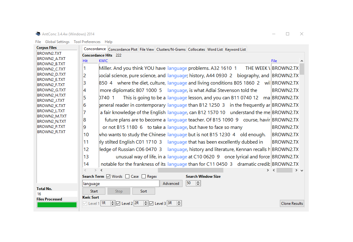
AntConc: The Standard for Teaching and Research
AntConc is the most widely used free concordancing tool, and for good reason:
Strengths:
- Completely free and cross-platform (Windows, Mac, Linux)
- No installation hassles or dependencies
- Intuitive interface ideal for beginners
- Powerful search capabilities including regex
- Beyond concordancing: collocates, clusters, keywords
- Handles large corpora efficiently
- Widely taught, extensive documentation
When to use AntConc:
- Teaching concordancing to students
- Quick exploratory analysis
- Working with local text files
- Classroom demonstrations
- Collaborative research (everyone can use the same tool)
- When you need quick results without coding
AntConc showing concordance lines for “language” with collocates panel
WordSmith Tools: The Professional Standard
WordSmith is commercial software that has long been the gold standard for corpus linguistics research.
Strengths:
- Comprehensive suite of interconnected tools
- Sophisticated statistical analysis built-in
- Dispersion plots show distribution across texts
- Keyword analysis identifies characteristic vocabulary
- Excellent documentation and tutorials
- Handles very large corpora
- Professional-quality visualizations
When to use WordSmith:
- Professional corpus linguistics research
- Publication-quality statistical analysis
- When budget allows (institutional licenses available)
- Complex multi-step workflows
- Teaching advanced corpus methods
Limitations:
- Costs money (though reasonable for professional tool)
- Windows only (though runs on Mac via Wine)
- Steeper learning curve than AntConc
- Still limited in reproducibility vs. scripting
SketchEngine: Web-Based Power
SketchEngine offers both web and desktop access with advanced features.
Strengths:
- Access to pre-loaded corpora in 90+ languages
- “Word Sketch” shows grammatical/collocational behavior at a glance
- Automatic corpus processing and annotation
- Terminology extraction for specialized fields
- Parallel corpora for translation studies
- Web interface means no installation
- Collaborative features for team projects
When to use SketchEngine:
- Multilingual research
- Need immediate access to large corpora
- Working with team members remotely
- Translation and terminology work
- When you want professional corpus preparation done for you
Limitations:
- Subscription based (though free trial available)
- Less control over corpus composition
- Learning curve for advanced features
- Depends on internet connection
Specialized Tools
ParaConc: Purpose-built for parallel texts (source + translation)
- Aligns source and target sentences
- Search both sides simultaneously
- Essential for translation studies
- More specialized than general tools
MONOCONC: Focused on monolingual concordancing with strong customization options
Web-Based Corpus Interfaces
Many large corpora are accessible through web interfaces, eliminating setup overhead.
BYU Corpora Family
Mark Davies’s suite includes industry-standard reference corpora:
COCA (Corpus of Contemporary American English):
- Over 1 billion words (1990-present)
- Balanced across genres (spoken, fiction, magazines, newspapers, academic)
- Updated annually
- Rich metadata for filtering
COHA (Corpus of Historical American English):
- 400+ million words (1820s-2000s)
- Track language change across two centuries
- Balanced by decade and genre
Other BYU Corpora:
- NOW Corpus (web, constantly updated)
- TV Corpus (soap operas)
- Movie Corpus
- Wikipedia Corpus
- And many more…
Strengths of BYU Corpora:
- Immediate access—no download or setup
- Professional corpus design
- Sophisticated search interface
- Metadata filtering (genre, date, etc.)
- Frequency/trend visualizations
- Free for academic use
When to use BYU Corpora:
- Quick checks of English usage
- Tracking diachronic change
- Comparing across genres
- Teaching with real data
- Exploring before building custom corpus
Limitations:
- Can’t upload your own texts
- English-focused (though some other languages available)
- Search options limited to interface
- Can’t save/export large result sets in free version
- Dependent on their corpus design decisions
COCA concordance for “language” showing genre distribution
Lextutor and Other Web Concordancers
Lextutor offers free web-based tools including concordancers, vocabulary profilers, and more.
When to use web concordancers:
- Classroom demonstrations (no installation)
- Quick vocabulary lookups
- Exploring concordancing concepts
- Public/shared computers
- Mobile devices
Programming-Based Solutions
For maximum flexibility, reproducibility, and integration with other analytical tools, programming languages offer unmatched power.
R with quanteda (Our Focus)
Why R and quanteda for concordancing:
Reproducibility:
- Scripts document every step
- Share exact methodology with colleagues
- Regenerate results precisely
- Satisfy open science requirements
- Version control with Git
Flexibility:
- Custom search patterns
- Unlimited filtering and grouping
- Integration with data manipulation (dplyr)
- Combine concordancing with statistics
- Automated workflows for large projects
Integration:
- Connect to databases
- Web scraping for corpus building
- Statistical modeling on results
- Machine learning pipelines
- Advanced visualization (ggplot2)
Scalability:
- Handle massive datasets
- Parallel processing for speed
- Cloud computing integration
- Automated batch processing
- Memory-efficient for large corpora
Cost:
- Completely free and open source
- No licensing fees ever
- Extensive package ecosystem
- Active development community
When to use R/quanteda:
- Reproducible research publications
- Complex analytical workflows
- Large-scale or custom corpora
- Integration with statistics/modeling
- Automated/repeating analyses
- When you need to document everything
Learning investment:
- Steeper initial learning curve than GUI tools
- Programming basics required
- But: transferable skills across research career
- Worth it for serious corpus work
- This tutorial will guide you!
Python with NLTK and Others
Python offers similar advantages through packages like NLTK, spaCy, and others.
When Python might be better:
- You already know Python
- Heavy NLP preprocessing needed
- Machine learning focus
- Web development integration
- You’re in a Python-centric community
For most linguistic concordancing, R/quanteda is excellent.
Features:
- Upload your own texts
- Pre-written code chunks (just click run)
- Modify code as you learn
- Download results (CSV, Excel)
- No installation needed
- Reproducible but accessible
When to use:
- Learning concordancing and coding together
- One-off analyses
- Quick results with your own texts
- Sharing with non-programmers
- Teaching hybrid approaches
Choosing the Right Tool
Different tasks call for different tools. Many researchers use multiple approaches:
Task
Recommended Tool
Why
Teaching basics
AntConc or Web interfaces
Zero barrier to entry, visual, immediate
Quick exploration
Web corpora (COCA, etc.)
No setup, instant results
Translation work
ParaConc or SketchEngine
Purpose-built for parallel texts
Publication research
WordSmith or R
Professional features, reproducibility
Large custom corpora
R/Python
Scalability, automation
Reproducible workflows
R/Python
Script everything, version control
Team projects
SketchEngine or R
Collaboration features
Learning to code
Our notebook tool
Gentle introduction
Pro tip: Start with AntConc or web interfaces to learn concepts, then graduate to R when you need more power or reproducibility.
Why Use R for Concordancing?
Given the excellent GUI tools available, why invest in learning R for concordancing?
The Reproducibility Imperative
Modern science increasingly demands reproducibility:
With GUI tools:
- “I opened AntConc, loaded corpus X, searched for Y, sorted by…”
- Hard to document exact steps
- Difficult for others to replicate
- Easy to forget what you did
With R scripts:
# Load corpus corpus <-readLines("my_texts.txt") # Create concordance kwic_result <- quanteda::kwic( tokens(corpus), pattern ="test_pattern", window =5) # Filter and arrange kwic_filtered <- kwic_result |>filter(str_detect(post, "specific_pattern")) |>arrange(pre) # Export write.csv(kwic_filtered, "results.csv")
Every step explicit
Exact replication possible
Share script with paper
Satisfies open science standards
Integration and Power
Seamless workflow:
# 1. Build corpus texts <-scrape_websites(urls) # 2. Concordance kwics <-kwic(tokens(texts), pattern) # 3. Statistical analysis collocation_test(kwics) # 4. Visualization ggplot(kwics) + ... # 5. Modeling regression_model <-lm(frequency ~ variables) # All in one environment!
vs. GUI approach:
- Export from concordancer
- Import to Excel
- Clean/rearrange
- Import to statistics software
- Export results
- Import to visualization tool
- Hope nothing was lost in translation!
Customization and Control
R allows:
- Custom search patterns beyond tool limitations
- Arbitrary filtering logic
- Novel analysis approaches
- Integration with your specific workflow
- Automation of repetitive tasks
- Handling of unusual data formats
Example: Complex filtering
# Find "must" but only:
# - In questions
# - Followed by a verb
# - Not in negation
# - In formal register

# Easy in R, impossible/tedious in GUI tools
You don’t need to be a programmer - basic R suffices for concordancing, and you’ll learn by doing.
When GUI Tools Are Better
Use GUI tools when:
- Quick one-off exploration
- Teaching complete beginners
- Working with non-technical collaborators
- You need results immediately
- The analysis is truly simple
- Learning R isn’t worth it for this project
But consider R when:
- Doing serious research
- Need reproducibility
- Complex or custom analysis
- Working with large corpora
- Building a research program
- Want transferable skills
Exercise 2.1: Tool Comparison
Hands-On Tool Exploration
Task: Search for the same pattern in the same text using two different tools.
Choose a simple text (e.g., a news article)
Search for a word (e.g., “government”)
Try in:
AntConc (download and use)
A web concordancer (e.g., Lextutor)
OR our R notebook tool
Compare:
- Which was easiest to set up?
- Which gave you most control?
- Which had best export options?
- Which would you use for what purposes?
Discuss:
- What are the trade-offs?
- When would each be appropriate?
- What features matter most to you?
Part 3: Getting Started with R Concordancing
Now we’ll move from theory to practice, learning to create concordances using R and the quanteda package.
Benefits:
- Clear what dependencies you have
- Others can see what they need to install
- Easier to troubleshoot if something’s missing
- Professional script organization
# Good practice
library(quanteda)
library(dplyr)
# ... rest of script

# Poor practice
# Code scattered throughout
library(quanteda)
# more code
library(dplyr)  # forgot earlier
# more code
Loading Your First Text
We’ll use Lewis Carroll’s Alice’s Adventures in Wonderland as our example text. This classic provides:
- Rich literary language
- Memorable characters and phrases
- Sufficient length for meaningful patterns
- Public domain (freely available)
Loading from Project Gutenberg
Project Gutenberg provides free access to thousands of public domain texts.
Code
# Load Alice's Adventures in Wonderland rawtext <-readLines("https://www.gutenberg.org/files/11/11-0.txt")
rawtext
*** START OF THE PROJECT GUTENBERG EBOOK 11 ***
[Illustration]
Alice’s Adventures in Wonderland
by Lewis Carroll
THE MILLENNIUM FULCRUM EDITION 3.0
Contents
CHAPTER I. Down the Rabbit-Hole
CHAPTER II. The Pool of Tears
CHAPTER III. A Caucus-Race and a Long Tale
CHAPTER IV. The Rabbit Sends in a Little Bill
CHAPTER V. Advice from a Caterpillar
CHAPTER VI. Pig and Pepper
CHAPTER VII. A Mad Tea-Party
CHAPTER VIII. The Queen’s Croquet-Ground
CHAPTER IX. The Mock Turtle’s Story
CHAPTER X. The Lobster Quadrille
CHAPTER XI. Who Stole the Tarts?
CHAPTER XII. Alice’s Evidence
CHAPTER I.
Down the Rabbit-Hole
Alice was beginning to get very tired of sitting by her sister on the
bank, and of having nothing to do: once or twice she had peeped into
the book her sister was reading, but it had no pictures or
conversations in it, “and what is the use of a book,” thought Alice
“without pictures or conversations?”
What just happened:
- readLines() fetched the text file from the web
- Each line became an element in a vector called rawtext
- We now have the complete book in R memory
Understanding the Raw Text Structure
Looking at the output, we see:
- Line 1-30: Title page, legal information, contents
- Real text starts: After “CHAPTER I”
- Formatting: Chapter headings, line breaks, spaces
This is typical of Project Gutenberg texts—they include metadata and formatting we need to handle.
Data Preparation: Cleaning the Text
Raw texts require preprocessing before analysis. This crucial step ensures clean, analysis-ready data.
Why Data Preparation Matters
The reality of text data:
- Downloaded texts include metadata (titles, licenses, etc.)
- Formatting varies (line breaks, spaces, special characters)
- Inconsistencies abound (encodings, punctuation)
- Structure needs standardization
Impact on analysis:
- Bad: Metadata contaminates results
- Bad: Formatting breaks pattern matching
- Bad: Inconsistencies cause missed matches
- Good: Clean data = reliable results
The 80/20 Rule of Text Analysis
Researchers often spend:
- 80% of time: Cleaning and preparing data
- 20% of time: Actually analyzing it
This isn’t wasted time—it’s essential investment. Poor preparation leads to unreliable results, wasted effort, and potentially wrong conclusions.
The payoff:
- Accurate results
- Reproducible analyses
- Confidence in findings
- Time saved troubleshooting later
Cleaning Alice in Wonderland
Let’s transform our raw text into analysis-ready format:
Code
text <- rawtext |># Collapse all lines into one continuous text paste0(collapse =" ") |># Remove extra white spaces (multiple spaces → single space) stringr::str_squish() |># Remove everything before "CHAPTER I." (title page, contents, etc.) stringr::str_remove(".*CHAPTER I\\.")
substr(text, start = 1, stop = 1000)
Down the Rabbit-Hole Alice was beginning to get very tired of sitting by her sister on the bank, and of having nothing to do: once or twice she had peeped into the book her sister was reading, but it had no pictures or conversations in it, “and what is the use of a book,” thought Alice “without pictures or conversations?” So she was considering in her own mind (as well as she could, for the hot day made her feel very sleepy and stupid), whether the pleasure of making a daisy-chain would be worth the trouble of getting up and picking the daisies, when suddenly a White Rabbit with pink eyes ran close by her. There was nothing so _very_ remarkable in that; nor did Alice think it so _very_ much out of the way to hear the Rabbit say to itself, “Oh dear! Oh dear! I shall be late!” (when she thought it over afterwards, it occurred to her that she ought to have wondered at this, but at the time it all seemed quite natural); but when the Rabbit actually _took a watch out of its waistcoat-pocke
What each step does:
1. paste0(collapse = " ")
- Joins all separate lines into one continuous string
- Why: Concordancing works better on continuous text
- Prevents artificial line-break effects on patterns
2. stringr::str_squish()
- Removes leading/trailing whitespace
- Reduces multiple spaces to single space
- Standardizes spacing throughout
3. stringr::str_remove(".*CHAPTER I\\.")
- Removes everything up to and including “CHAPTER I.”
- .* means “any characters”
- \\. means a literal period (escaped)
- Isolates the actual story text
Understanding the Regular Expression
The pattern ".*CHAPTER I\\." breaks down as:
. = any character
* = zero or more times
CHAPTER I = literal text
\\. = escaped period (. is special in regex)
Together: “Match any amount of any characters, followed by ‘CHAPTER I.’”
Regular expressions are powerful pattern-matching tools we’ll explore more later!
Exercise 3.1: Text Preparation Practice
Clean Your Own Text
Load a different Project Gutenberg text:
Code
# Example: Pride and Prejudice raw_pride <-readLines("https://www.gutenberg.org/files/1342/1342-0.txt")
Your tasks:
1. Examine the first 50 lines—what needs removing?
2. Find where the actual text starts (look for “Chapter” or similar)
3. Clean the text using the Alice example as a model
4. Verify your result looks correct
Questions:
- What patterns did you use to identify the start of the text?
- Were there any challenges specific to this text?
- How would you generalize this cleaning procedure?
Bonus: Write a function that automates Gutenberg text cleaning:
Code
clean_gutenberg <-function(url, start_pattern) { # Your code here }
Part 4: Creating Your First Concordance
Now that we have clean text, let’s extract our first concordances!
Basic KWIC Extraction
The kwic() function from quanteda makes concordancing straightforward.
Your First Concordance
Let’s search for “Alice”:
Code
mykwic <- quanteda::kwic( quanteda::tokens(text), # Tokenize the text first pattern = quanteda::phrase("Alice")) |># What to search for as.data.frame() # Convert to data frame
docname
from
to
pre
keyword
post
pattern
text1
4
4
Down the Rabbit-Hole
Alice
was beginning to get very
Alice
text1
63
63
a book , ” thought
Alice
“ without pictures or conversations
Alice
text1
143
143
in that ; nor did
Alice
think it so _very_ much
Alice
text1
229
229
and then hurried on ,
Alice
started to her feet ,
Alice
text1
299
299
In another moment down went
Alice
after it , never once
Alice
text1
338
338
down , so suddenly that
Alice
had not a moment to
Alice
Success! You’ve created your first concordance. Let’s understand what happened.
Understanding the kwic() Function
Function structure:
kwic(
  x =,        # The tokenized text
  pattern =,  # What to search for
  window =,   # Context size (default: 5)
  ...         # Other options
)
Required arguments:
- x: Must be a tokens object (created by tokens())
- pattern: What you’re searching for
Important pattern specification:
- quanteda::phrase("Alice") = exact phrase (case-sensitive)
- Without phrase(), searches for individual tokens
- We’ll explore more pattern types soon!
The Concordance Table Structure
The result is a data frame with these columns:
Column
Contains
Purpose
docname
Document name
Track source (useful for multi-text corpora)
from
Start position
Where match begins (token number)
to
End position
Where match ends
pre
Left context
Words before the keyword
keyword
The match
Your search term
post
Right context
Words after the keyword
pattern
Search pattern
What you searched for (useful when searching multiple patterns)
Exploring Your Concordance
How many matches did we find?
Code
nrow(mykwic) # Count rows
[1] 386
OR
Code
length(mykwic$keyword) # Count keywords
[1] 386
We found 386 instances of “Alice” in the text!
What variations were found?
Code
table(mykwic$keyword)
Alice
  386
All instances are exactly “Alice” (case-sensitive match).
Adjusting the Context Window
The default context is 5 words on each side. Sometimes you need more:
“ without pictures or conversations ? ” So she was
alice
text1
143
143
was nothing so _very_ remarkable in that ; nor did
Alice
think it so _very_ much out of the way to
alice
text1
229
229
and looked at it , and then hurried on ,
Alice
started to her feet , for it flashed across her
alice
text1
299
299
rabbit-hole under the hedge . In another moment down went
Alice
after it , never once considering how in the world
alice
text1
338
338
, and then dipped suddenly down , so suddenly that
Alice
had not a moment to think about stopping herself before
alice
When to use wider windows:
- Understanding full sentence context
- Analyzing longer constructions
- Studying distant relationships
- Literary analysis requiring more text
When to use narrower windows:
- Focused on immediate collocates
- Large result sets (easier to scan)
- Identifying local patterns
- Quick exploration
Choosing Context Window Size
General guidelines:
- 5 words (default): Good starting point for most analyses
- 3 words: Immediate collocates, tight focus
- 10-15 words: Sentence-level context
- 20+ words: Paragraph-level context (rare, usually too much)
Experiment! Try different sizes and see what reveals patterns best for your research question.
Exercise 4.1: Basic Concordancing Practice
Your Turn!
Using the Alice text, complete these tasks:
1. Extract concordances for “confused”
Answer
Code
kwic_confused <- quanteda::kwic( x = quanteda::tokens(text), pattern = quanteda::phrase("confused") ) # Display first 10 kwic_confused |>as.data.frame() |>head(10)
  docname  from    to                    pre  keyword
1   text1  6217  6217     , calling out in a confused
2   text1 19140 19140     . ” This answer so confused
3   text1 19325 19325 said Alice , very much confused
4   text1 33422 33422      she knew ) to the confused
                                 post  pattern
1                    way , “ Prizes ! confused
2               poor Alice , that she confused
3                   , “ I don’t think confused
4 clamour of the busy farm-yard—while confused
2. How many times does “wondering” appear?
Answer
Code
quanteda::kwic( x = quanteda::tokens(text), pattern = quanteda::phrase("wondering") ) |>as.data.frame() |>nrow()
[1] 7
There are 7 instances.
3. Extract “strange” with a 7-word window, show first 5 lines
  docname  from    to                                    pre keyword
1   text1  3527  3527     , but her voice sounded hoarse and strange
2   text1 13147 13147        right size , that it felt quite strange
3   text1 32997 32997    she could remember them , all these strange
4   text1 33204 33204 place around her became alive with the strange
5   text1 33514 33514      eyes bright and eager with many a strange
                                      post pattern
1             , and the words did not come strange
2              at first ; but she got used strange
3    Adventures of hers that you have just strange
4 creatures of her little sister’s dream . strange
5       tale , perhaps even with the dream strange
Challenge: Pick your own word and explore different window sizes. Which size reveals the most about how the word is used?
Part 5: Exporting and Saving Concordances
Once you’ve created concordances, you’ll often want to save them for further analysis, sharing, or documentation.
Exporting to Excel
Excel spreadsheets are widely compatible and easy to share with colleagues.
Code
# Export to Excel
write_xlsx(mykwic, here::here("my_alice_concordance.xlsx"))
What this does:
- write_xlsx() creates an Excel file (.xlsx)
- here::here() saves it in your working directory
- Result: A spreadsheet with all concordance data
Using here() for File Paths
The here package makes file paths easier and more portable:
Code
# Without here - breaks if you move project
write_xlsx(data, "C:/Users/YourName/Documents/project/file.xlsx")

# With here - works anywhere
write_xlsx(data, here::here("file.xlsx"))

# Subdirectories
write_xlsx(data, here::here("output", "results", "file.xlsx"))
Benefits:
- Works on Windows, Mac, Linux
- No hard-coded paths
- Project-relative paths
- Collaborators can run your code
Other Export Formats
Code
# CSV (universal, simple) write.csv(mykwic, here::here("concordance.csv"), row.names =FALSE) # Tab-separated (good for large texts) write.table(mykwic, here::here("concordance.txt"), sep ="\t", row.names =FALSE) # R data format (preserves all R attributes) saveRDS(mykwic, here::here("concordance.rds")) # Load RDS back later mykwic_loaded <-readRDS(here::here("concordance.rds"))
When to use each:
Format
Best For
Why
Excel (.xlsx)
Sharing with non-R users
Widely compatible, can open directly
CSV
Simple data exchange
Universal, plain text, version control friendly
TSV/TXT
Very large datasets
Smaller file size than Excel
RDS
R-to-R sharing
Preserves all object attributes, efficient
Creating Export-Ready Tables
For presentations or reports, format your concordances nicely:
Code
# Create a nicely formatted subset mykwic |>head(20) |># First 20 for manageable size select(pre, keyword, post) |># Just the interesting columns flextable() |>set_caption("Concordance of 'Alice' in Alice's Adventures in Wonderland") |>theme_zebra() |>autofit() |>save_as_docx(path = here::here("concordance_table.docx"))
This creates a Word document with a professional-looking table—perfect for embedding in papers!
Part 6: Advanced Pattern Matching
Multi-Word Expressions and Phrases
While single words are common search targets, language research often requires extracting phrases or multi-word expressions (MWEs).
Why Multi-Word Expressions Matter
Language is more than individual words:
- Idioms: “kick the bucket”, “spill the beans”
- Collocations: “strong coffee”, “make a decision”
- Fixed expressions: “by and large”, “as a matter of fact”
- Titles and names: “Mad Hatter”, “Cheshire Cat”
- Technical terms: “global warming”, “machine learning”
These MWEs often function as single semantic units despite containing multiple words. Searching for individual words misses the unified meaning.
Extracting Phrases with quanteda
The phrase() function tells quanteda to treat multiple words as a single search unit:
Code
# Search for "poor alice" as a phrase kwic_pooralice <- quanteda::kwic( quanteda::tokens(text), pattern = quanteda::phrase("poor alice")) |>as.data.frame()
docname
from
to
pre
keyword
post
pattern
text1
1,541
1,542
go through , ” thought
poor Alice
, “ it would be
poor alice
text1
2,130
2,131
; but , alas for
poor Alice
! when she got to
poor alice
text1
2,332
2,333
use now , ” thought
poor Alice
, “ to pretend to
poor alice
text1
2,887
2,888
to the garden door .
Poor Alice
! It was as much
poor alice
text1
3,604
3,605
right words , ” said
poor Alice
, and her eyes filled
poor alice
text1
6,876
6,877
mean it ! ” pleaded
poor Alice
. “ But you’re so
poor alice
text1
7,290
7,291
more ! ” And here
poor Alice
began to cry again ,
poor alice
text1
8,239
8,240
at home , ” thought
poor Alice
, “ when one wasn’t
poor alice
text1
11,788
11,789
to it ! ” pleaded
poor Alice
in a piteous tone .
poor alice
text1
19,141
19,142
” This answer so confused
poor Alice
, that she let the
poor alice
What phrase() does:
- Treats “poor alice” as an inseparable unit
- Both words must appear consecutively
- Respects word boundaries
- Case-sensitive by default
Without phrase():
Code
# This would match "poor" and "alice" separately, anywhere in the text kwic(tokens(text), pattern =c("poor", "alice"))
Case Sensitivity Control
By default, searches are case-sensitive. Control this behavior:
Use case-insensitive when:
- Names might be capitalized variably
- Sentence-initial position matters
- Historical texts with inconsistent capitalization
- You want all variants regardless of position
Keep case-sensitive when:
- Proper names vs. common words matter (e.g., “Apple” vs. “apple”)
- You’re studying capitalization patterns
- Precision is more important than recall
Searching Multiple Phrases
Search for several phrases simultaneously:
Code
# Search for multiple character descriptions patterns <-c("poor alice", "little alice", "dear alice") kwic_alice_variants <- quanteda::kwic( quanteda::tokens(text), pattern =phrase(patterns) ) |>as.data.frame() # See which variants were found table(kwic_alice_variants$keyword)
   docname  from    to                    pre    keyword
1    text1 16576 16577   wish I’d gone to see the Hatter
2    text1 16607 16608 and the March Hare and the Hatter
3    text1 16859 16860 wants cutting , ” said the Hatter
4    text1 16905 16906     it’s very rude . ” The Hatter
5    text1 17049 17050         a bit ! ” said the Hatter
6    text1 17174 17175      with you , ” said the Hatter
7    text1 17209 17210  , which wasn’t much . The Hatter
8    text1 17287 17288  days wrong ! ” sighed the Hatter
9    text1 17338 17339         in as well , ” the Hatter
10   text1 17453 17454 should it ? ” muttered the Hatter
                          post    pattern
1      instead ! ” CHAPTER VII the hatter
2        were having tea at it the hatter
3        . He had been looking the hatter
4    opened his eyes very wide the hatter
5           . “ You might just the hatter
6  , and here the conversation the hatter
7       was the first to break the hatter
8               . “ I told you the hatter
9   grumbled : “ you shouldn’t the hatter
10       . “ Does _your_ watch the hatter
  docname  from    to               pre keyword                     post
1   text1   932   933   ! ” ( Dinah was the cat             . ) “ I hope
2   text1 15624 15625 a few yards off . The Cat only grinned when it saw
3   text1 15749 15750   get to , ” said the Cat         . “ I don’t much
4   text1 15775 15776   you go , ” said the Cat            . “ — so long
5   text1 15805 15806  do that , ” said the Cat          , “ if you only
  pattern
1 the cat
2 the cat
3 the cat
4 the cat
5 the cat
Challenge: Find all instances of character names with titles (e.g., “the Duchess”, “the King”, “the Queen”). How would you search for these patterns efficiently?
Part 7: Regular Expressions for Power Users
Regular expressions (regex) provide powerful pattern-matching capabilities beyond exact words or phrases.
Understanding Regular Expressions
A regular expression is a sequence of characters that describes a search pattern. Think of it as a wildcard on steroids.
Why Regular Expressions Matter
Without regex:
- Search for “walk”, “walks”, “walked”, “walking” separately
- Four searches, combine results manually
- Miss any variants you didn’t think of
With regex:
- "walk.*" finds all forms in one search
- Captures “walks”, “walked”, “walking”, “walker”, etc.
- Systematic, comprehensive
Regular Expression Types
There are three fundamental categories:
1. Symbols for Frequencies
These control how many times a pattern appears:
Symbol
Explanation
Example
?
Preceding item is optional (0 or 1 times)
walk[a-z]? → walk, walks
*
Preceding item appears 0 or more times
walk[a-z]* → walk, walks, walked, walking
+
Preceding item appears 1 or more times
walk[a-z]+ → walks, walked, walking (not walk)
{n}
Preceding item appears exactly n times
walk[a-z]{2} → walked
{n,}
Preceding item appears n or more times
walk[a-z]{2,} → walked, walking
{n,m}
Preceding item appears n to m times
walk[a-z]{2,3} → walked, walking
2. Character Classes
These represent groups of characters:
Symbol
Explanation
[ab]
Lowercase a or b
[AB]
Uppercase A or B
[12]
Digits 1 or 2
[:digit:]
Any digit: 0-9
[:lower:]
Any lowercase letter: a-z
[:upper:]
Any uppercase letter: A-Z
[:alpha:]
Any letter: a-z, A-Z
[:alnum:]
Any letter or digit
[:punct:]
Any punctuation character
[:space:]
Any whitespace (space, tab, newline)
.
Any single character (wildcard)
3. Position Anchors
These specify where patterns must appear:
Symbol
Explanation
\\b
Word boundary (start or end of word)
\\B
Not a word boundary (inside a word)
^
Start of string/line
$
End of string/line
<
Start of word
>
End of word
Using Regular Expressions in Concordancing
To use regex in kwic(), set valuetype = "regex":
Code
# Find words starting with "alic" OR "hatt" patterns <-"\\b(alic|hatt).*"kwic_regex <- quanteda::kwic( quanteda::tokens(text), pattern = patterns, valuetype ="regex") |>as.data.frame()
docname
from
to
pre
keyword
post
pattern
text1
4
4
Down the Rabbit-Hole
Alice
was beginning to get very
\b(alic|hatt).*
text1
63
63
a book , ” thought
Alice
“ without pictures or conversations
\b(alic|hatt).*
text1
143
143
in that ; nor did
Alice
think it so _very_ much
\b(alic|hatt).*
text1
229
229
and then hurried on ,
Alice
started to her feet ,
\b(alic|hatt).*
text1
299
299
In another moment down went
Alice
after it , never once
\b(alic|hatt).*
text1
338
338
down , so suddenly that
Alice
had not a moment to
\b(alic|hatt).*
text1
521
521
“ Well ! ” thought
Alice
to herself , “ after
\b(alic|hatt).*
text1
647
647
for , you see ,
Alice
had learnt several things of
\b(alic|hatt).*
text1
719
719
got to ? ” (
Alice
had no idea what Latitude
\b(alic|hatt).*
text1
910
910
else to do , so
Alice
soon began talking again .
\b(alic|hatt).*
Pattern breakdown:
- \\b = word boundary (start of word)
- (alic|hatt) = either “alic” OR “hatt”
- .* = followed by any characters
- Result: “alice”, “hatter”, “hatters” but NOT “malice” or “shatter”
Common Regex Patterns for Concordancing
Find all forms of a word:
Code
# All forms of "think" kwic(tokens(text), pattern ="\\bthink.*", valuetype ="regex") # Matches: think, thinks, thinking, thought, thinker # Words ending in "ing" kwic(tokens(text), pattern =".*ing\\b", valuetype ="regex") # Words ending in "tion" kwic(tokens(text), pattern =".*tion\\b", valuetype ="regex")
Find words of specific length:
Code
# Three-letter words kwic(tokens(text), pattern ="\\b[a-z]{3}\\b", valuetype ="regex") # Words 10+ letters long kwic(tokens(text), pattern ="\\b[a-z]{10,}\\b", valuetype ="regex")
Find patterns with specific structure:
Code
# Words with double letters kwic(tokens(text), pattern ="\\b\\w*(.)\\1\\w*\\b", valuetype ="regex") # Matches: little, bottle, matters, etc. # Words starting with vowels kwic(tokens(text), pattern ="\\b[aeiou]\\w*", valuetype ="regex")
Regex Can Be Tricky!
Regular expressions are powerful but can be:
- Cryptic: \\b(?:alic|hatt).* looks like gibberish at first
- Fragile: Small changes can break patterns
- Surprising: They might match more (or less) than you expect
Best practices:
- Test patterns on small samples first
- Use online regex testers (regex101.com)
- Comment your patterns explaining what they do
- Start simple, add complexity gradually
- Check results carefully—regex can surprise you!
[1] docname from    to      pre     keyword post    pattern
<0 rows> (or 0-length row.names)
2. How many words begin with “pit”?
Answer
Code
quanteda::kwic( x = quanteda::tokens(text), pattern ="\\bpit.*", valuetype ="regex") |>as.data.frame() |>nrow()
[1] 5
3. Find words ending in “ption” (first 5)
Answer
Code
quanteda::kwic( x = quanteda::tokens(text), pattern =".*ption\\b", valuetype ="regex") |>as.data.frame() |>head(5)
  docname from   to                         pre  keyword
1   text1 5775 5775 adjourn , for the immediate adoption
                          post    pattern
1 of more energetic remedies — .*ption\\b
Challenge:
1. Find all words starting with “un-” (negative prefix)
2. Find all words with exactly 4 letters
3. Find all words containing “qu”
4. Find words that appear to be capitalized names (hint: uppercase start)
Part 8: Filtering and Refining Concordances
Raw concordances are just the starting point. The real power comes from filtering, sorting, and refining results to reveal patterns.
Piping for Conditional Concordances
Often we want concordances only when specific conditions are met. Piping with dplyr makes this elegant.
The Pipe Operator: |> or %>%
Piping chains operations together: “do this, then do that”
Code
# Without piping (nested, hard to read) filter(as.data.frame(kwic(tokens(text), "alice")), condition) # With piping (clear, sequential) kwic(tokens(text), "alice") |>as.data.frame() |>filter(condition) # Read as: "take text, make concordance, convert to dataframe, filter"
Filtering by Context
Find “alice” only when preceded by “poor” or “little”:
Code
quanteda::kwic( x = quanteda::tokens(text), pattern ="alice") |>as.data.frame() |># Filter: "pre" column must end with "poor" or "little" dplyr::filter(stringr::str_detect(pre, "poor$|little$")) -> kwic_pipe
docname
from
to
pre
keyword
post
pattern
text1
1,542
1,542
through , ” thought poor
Alice
, “ it would be
alice
text1
1,725
1,725
” but the wise little
Alice
was not going to do
alice
text1
2,131
2,131
but , alas for poor
Alice
! when she got to
alice
text1
2,333
2,333
now , ” thought poor
Alice
, “ to pretend to
alice
text1
3,605
3,605
words , ” said poor
Alice
, and her eyes filled
alice
text1
6,877
6,877
it ! ” pleaded poor
Alice
. “ But you’re so
alice
text1
7,291
7,291
! ” And here poor
Alice
began to cry again ,
alice
text1
8,240
8,240
home , ” thought poor
Alice
, “ when one wasn’t
alice
text1
11,789
11,789
it ! ” pleaded poor
Alice
in a piteous tone .
alice
text1
19,142
19,142
This answer so confused poor
Alice
, that she let the
alice
Pattern breakdown:
- str_detect(pre, "poor$|little$")
- Check if pre (preceding context) contains…
- poor$ = “poor” at the end ($ = end anchor)
- | = OR
- little$ = “little” at the end
Why the $ matters:
- "poor$" = must be last word before keyword
- "poor" = anywhere in preceding context
- Precision prevents false matches like “poorly alice”
Multiple Conditions
Combine filters for complex queries:
Code
kwic(tokens(text), "said") |>as.data.frame() |># Must be preceded by name AND followed by specific punctuation filter( str_detect(pre, "Alice$|Hatter$|Queen$"), str_detect(post, "^,|^\\.") )
This finds speech acts: “[Character] said, …”
Filtering by Position
Find instances only at specific positions in the text:
Code
kwic(tokens(text), "alice") |>as.data.frame() |># Only in first 1000 tokens filter(from <=1000) # Only in last quarter of text max_position <-max(from) kwic_data |>filter(from >= max_position *0.75)
Sorting and Arranging Concordances
Reordering concordances reveals patterns invisible in occurrence order.
Alphabetical Sorting
Sort by what follows the keyword:
Code
quanteda::kwic( x = quanteda::tokens(text), pattern ="alice") |>as.data.frame() |># Arrange alphabetically by following context dplyr::arrange(post) -> kwic_ordered
docname
from
to
pre
keyword
post
pattern
text1
7,754
7,754
happen : “ ‘ Miss
Alice
! Come here directly ,
alice
text1
2,888
2,888
the garden door . Poor
Alice
! It was as much
alice
text1
2,131
2,131
but , alas for poor
Alice
! when she got to
alice
text1
30,891
30,891
voice , the name “
Alice
! ” CHAPTER XII .
alice
text1
8,423
8,423
“ Oh , you foolish
Alice
! ” she answered herself
alice
text1
2,606
2,606
and curiouser ! ” cried
Alice
( she was so much
alice
text1
25,861
25,861
I haven’t , ” said
Alice
) — “ and perhaps
alice
text1
32,275
32,275
explain it , ” said
Alice
, ( she had grown
alice
text1
32,843
32,843
for you ? ” said
Alice
, ( she had grown
alice
text1
1,678
1,678
here before , ” said
Alice
, ) and round the
alice
Why sort alphabetically?
- Groups similar contexts together
- Reveals collocational patterns
- Makes manual analysis easier
- Identifies semantic prosody
Sort by different columns:
Code
arrange(pre)    # By preceding context
arrange(keyword)  # By matched pattern (if searching multiple)
arrange(from)     # By position in text (chronological)
Sorting by Frequency
More powerful: arrange by how common collocates are.
Step-by-Step Frequency Sorting
Code
quanteda::kwic( x = quanteda::tokens(text), pattern ="alice") |>as.data.frame() |># Extract first word after keyword dplyr::mutate(post1 =str_remove_all(post, " .*")) |># Group by that word dplyr::group_by(post1) |># Count frequency of each dplyr::mutate(post1_freq =n()) |># Sort by frequency (descending) dplyr::arrange(-post1_freq) -> kwic_ordered_coll
docname
from
to
pre
keyword
post
pattern
post1
post1_freq
text1
1,542
1,542
through , ” thought poor
Alice
, “ it would be
alice
,
78
text1
1,678
1,678
here before , ” said
Alice
, ) and round the
alice
,
78
text1
2,333
2,333
now , ” thought poor
Alice
, “ to pretend to
alice
,
78
text1
2,410
2,410
eat it , ” said
Alice
, “ and if it
alice
,
78
text1
2,739
2,739
to them , ” thought
Alice
, “ or perhaps they
alice
,
78
text1
2,945
2,945
of yourself , ” said
Alice
, “ a great girl
alice
,
78
text1
3,605
3,605
words , ” said poor
Alice
, and her eyes filled
alice
,
78
text1
3,751
3,751
oh dear ! ” cried
Alice
, with a sudden burst
alice
,
78
text1
3,918
3,918
narrow escape ! ” said
Alice
, a good deal frightened
alice
,
78
text1
4,181
4,181
so much ! ” said
Alice
, as she swam about
alice
,
78
What each step does:
mutate(post1 = str_remove_all(post, " .*"))
Creates new column post1
Extracts just the first word after keyword
Removes everything after first space
group_by(post1)
Groups all rows with same following word
Enables per-group calculations
mutate(post1_freq = n())
Counts how many in each group
n() returns group size
Adds frequency to each row
arrange(-post1_freq)
Sorts by frequency
- means descending (highest first)
Most common collocates appear first
Why frequency sorting matters:
- Reveals strongest collocational patterns
- Identifies typical vs. unusual usage
- Quantifies intuitions
- Prioritizes analysis (examine common patterns first)
Multi-Level Sorting
Sort by multiple criteria:
Code
kwic_data |>arrange(-post1_freq, -post2_freq, pre1) # Read as: "sort by post1 frequency (desc), # then post2 frequency (desc), # then pre1 (ascending)"
Extracting N-grams Around Keywords
Sometimes you want to analyze not just the next word, but the next 2-3 words (bigrams, trigrams).
Code
mykwic |>rowwise() |>mutate( # First word after post1 =unlist(strsplit(post, " "))[1], # Second word after post2 =unlist(strsplit(post, " "))[2], # Third word after post3 =unlist(strsplit(post, " "))[3], # Last word before pre1 =tail(unlist(strsplit(pre, " ")), 1), # Second-to-last before pre2 =tail(unlist(strsplit(pre, " ")), 2)[1], # Third-to-last before pre3 =tail(unlist(strsplit(pre, " ")), 3)[1] )
This creates columns for analyzing collocational patterns at different distances.
Exercise 8.1: Filtering and Sorting
Advanced Concordance Manipulation
Using the Alice text:
1. Find “said” preceded by a character name
Hint: Filter for names ending the pre context
Answer
Code
quanteda::kwic( x = quanteda::tokens(text), pattern ="said") |>as.data.frame() |>filter(str_detect(pre, "Alice$|Hatter$|Queen$|King$|Cat$")) |>head(10)
   docname  from    to                          pre keyword
1    text1  7715  7715           it seems , ” Alice    said
2    text1 11677 11677 said the Caterpillar . Alice    said
3    text1 14187 14187          that soup ! ” Alice    said
4    text1 14421 14421            that do , ” Alice    said
5    text1 15850 15850        direction , ” the Cat    said
6    text1 16894 16894   personal remarks , ” Alice    said
7    text1 17618 17618           yet ? ” the Hatter    said
8    text1 17747 17747         don’t ! ” the Hatter    said
9    text1 18857 18857              go on ! ” Alice    said
10   text1 19107 19107           the well , ” Alice    said
                                post pattern
1                  to herself , “ to    said
2            nothing : she had never    said
3               to herself , as well    said
4      very politely , feeling quite    said
5             , waving its right paw    said
6             with some severity ; “    said
7           , turning to Alice again    said
8  , tossing his head contemptuously    said
9                  very humbly ; “ I    said
10             to the Dormouse , not    said
2. Sort “and” concordances by preceding word frequency
# A tibble: 10 × 9
# Groups:   pre1 [1]
   docname  from    to pre                 keyword post  pattern pre1  pre1_freq
   <chr>   <int> <int> <chr>               <chr>   <chr> <fct>   <chr>     <int>
 1 text1      20    20 sister on the bank… and     of h… and     <NA>        642
 2 text1      52    52 conversations in i… and     what… and     <NA>        642
 3 text1     219   219 out of its waistco… and     look… and     <NA>        642
 4 text1     224   224 and looked at it ,  and     then… and     <NA>        642
 5 text1     263   263 take out of it ,    and     burn… and     <NA>        642
 6 text1     276   276 the field after it… and     fort… and     <NA>        642
 7 text1     329   329 tunnel for some wa… and     then… and     <NA>        642
 8 text1     431   431 sides of the well , and     noti… and     <NA>        642
 9 text1     662   662 lessons in the sch… and     thou… and     <NA>        642
10 text1     840   840 or Australia ? ” (  and     she … and     <NA>        642
Challenge: Find all instances of “very” followed by an adjective. How would you identify adjectives? (Hint: might need manual classification or a part-of-speech tagger)
Part 9: Working with Transcripts
Spoken language transcripts require special handling due to their unique features: speaker turns, pauses, laughter, overlaps, and other paralinguistic information.
Understanding Transcript Structure
Transcripts differ from written texts in important ways:
Written text:
- Continuous prose
- Standard punctuation
- Paragraph structure
- Edited and polished
<S1A-001$A> <#> Well how did the riding go tonight
<S1A-001$B> <#> It was good so it was <#> Just I I couldn't believe that she was going to let me jump <,> that was only the fourth time you know <#> It was great <&> laughter </&>
<S1A-001$A> <#> What did you call your horse
<S1A-001$B> <#> I can't remember <#> Oh Mary 's Town <,> oh
<S1A-001$A> <#> And how did Mabel do
<S1A-001$B> <#> Did you not see her whenever she was going over the jumps <#> There was one time her horse refused and it refused three times <#> And then <,> she got it round and she just lined it up straight and she just kicked it and she hit it with the whip <,> and over it went the last time you know <#> And Stephanie told her she was very determined and very well-ridden <&> laughter </&> because it had refused the other times you know <#> But Stephanie wouldn't let her give up on it <#> She made her keep coming back and keep coming back <,> until <,> it jumped it you know <#> It was good
<S1A-001$A> <#> Yeah I 'm not so sure her jumping 's improving that much <#> She uh <,> seemed to be holding the reins very tight
Transcript features visible:
- <S1A-001 Riding> = Header with file ID and title
- <I> = Transcript start marker
- <S1A-001$A> = Speaker A in file 001, section S1A
- <#> = Speech unit boundary
- <,> = Pause
- <&> laughter </&> = Paralinguistic information
Preprocessing Transcripts
Transcripts need different preprocessing than written texts.
Remove:
- Headers and metadata (usually)
- Markup that interferes with searching
- Excess spacing
It depends on your research question!
Collapsing Transcripts
For basic concordancing, collapse into continuous text:
Code
transcripts_collapsed <-sapply(files, function(x) { x <-readLines(x) # Collapse all lines together x <-paste0(x, collapse =" ") # Clean up spacing x <-str_squish(x) })
<S1A-001 Riding> <I> <S1A-001$A> <#> Well how did the riding go tonight <S1A-001$B> <#> It was good so it was <#> Just I I couldn't believe that she was going to let me jump <,> that was only the fourth time you know <#> It was great <&> laughter </&> <S1A-001$A> <#> What did you call your horse <S1A-001$B> <#> I can't remember <#> Oh Mary 's Town <,> oh <S1A-001$A> <#> And how did Mabel do <S1A-001$B> <#> Did you not see her whenever she was going over the jumps <#> There was one time her horse
<S1A-002 Dinner chat 1> <I> <S1A-002$A> <#> He 's been married for three years and is now <{> <[> getting divorced </[> <S1A-002$B> <#> <[> No no </[> </{> he 's got married last year and he 's getting <{> <[> divorced </[> <S1A-002$A> <#> <[> He 's now </[> </{> getting divorced <S1A-002$C> <#> Just right <S1A-002$D> <#> A wee girl of her age like <S1A-002$E> <#> Well there was a guy <S1A-002$C> <#> How long did she try it for <#> An hour a a year <S1A-002$B> <#> Mhm <{> <[> mhm </[> <S1A-002$E
<S1A-003 Dinner chat 2> <I> <S1A-003$A> <#> I <.> wa </.> I want to go to Peru but uh <S1A-003$B> <#> Do you <S1A-003$A> <#> Oh aye <S1A-003$B> <#> I 'd love to go to Peru <S1A-003$A> <#> I want I want to go up the Machu Picchu before it falls off the edge of the mountain <S1A-003$B> <#> Lima 's supposed to be a bit dodgy <S1A-003$A> <#> Mm <S1A-003$B> <#> Bet it would be <S1A-003$B> <#> Mm <S1A-003$A> <#> But I I just I I would like <,> Machu Picchu is collapsing <S1A-003$B> <#> I don't know wh
<S1A-004 Nursing home 1> <I> <S1A-004$A> <#> Honest to God <,> I think the young ones <#> Sure they 're flying on Monday in I think it 's Shannon <#> This is from Texas <S1A-004$B> <#> This English girl <S1A-004$A> <#> The youngest one <,> the dentist <,> she 's married to the dentist <#> Herself and her husband <,> three children and she 's six months pregnant <S1A-004$C> <#> Oh God <S1A-004$B> <#> And where are they going <S1A-004$A> <#> Coming to Dublin to the mother <{> <[> or <unclear> 3 sy
<S1A-005 Masons> <I> <S1A-005$A> <#> Right shall we risk another beer or shall we try and <,> <{> <[> ride the bikes down there or do something like that </[> <S1A-005$B> <#> <[> Well <,> what about the </[> </{> provisions <#> What time <{> <[> <unclear> 4 sylls </unclear> </[> <S1A-005$C> <#> <[> Is is your </[> </{> man coming here <S1A-005$B> <#> <{> <[> Yeah </[> <S1A-005$A> <#> <[> He said </[> </{> he would meet us here <S1A-005$B> <#> Just the boat 's arriving you know a few minutes ' wa
Concordancing Transcripts
Now extract concordances, being mindful of markup:
Code
kwic_trans <- quanteda::kwic( # Tokenize by whitespace to preserve markup quanteda::tokens(transcripts_collapsed, what ="fasterword"), # Search for "you know" pattern = quanteda::phrase("you know"), # Wider context for spoken language window =10) |>as.data.frame() |># Clean up file names dplyr::mutate(docname =str_replace_all(docname, ".*/(.*?).txt", "\\1"))
docname
from
to
pre
keyword
post
pattern
S1A-001
42
43
let me jump <,> that was only the fourth time
you know
<#> It was great <&> laughter </&> <S1A-001$A> <#> What
you know
S1A-001
140
141
the whip <,> and over it went the last time
you know
<#> And Stephanie told her she was very determined and
you know
S1A-001
164
165
<&> laughter </&> because it had refused the other times
you know
<#> But Stephanie wouldn't let her give up on it
you know
S1A-001
193
194
and keep coming back <,> until <,> it jumped it
you know
<#> It was good <S1A-001$A> <#> Yeah I 'm not
you know
S1A-001
402
403
'd be far better waiting <,> for that one <,>
you know
and starting anew fresh <S1A-001$A> <#> Yeah but I mean
you know
S1A-001
443
444
the best goes top of the league <,> <{> <[>
you know
</[> <S1A-001$A> <#> <[> So </[> </{> it 's like
you know
S1A-001
484
485
I 'm not sure now <#> We didn't discuss it
you know
<S1A-001$A> <#> Well it sounds like more money <S1A-001$B> <#>
you know
S1A-001
598
599
on Monday and do without her lesson on Tuesday <,>
you know
<#> But I was keeping her going cos I says
you know
S1A-001
727
728
to take it tomorrow <,> that she could take her
you know
the wee shoulder bag she has <S1A-001$A> <#> Mhm <S1A-001$B>
you know
S1A-001
808
809
<,> and <,> sort of show them around <,> uhm
you know
their timetable and <,> give them their timetable and show
you know
Key considerations:
what = "fasterword"
- Tokenizes by whitespace
- Preserves tags like <#>, <,>
- Alternative to default tokenization
Wider window (10 tokens)
- Spoken language has more fillers, pauses
- Need more context to understand utterance
- Captures more of the conversational flow
Why study “you know”?
- Discourse marker in spoken English
- Not about knowledge—about interaction
- Signals common ground, turn-taking
- Varies by speaker, context, genre
Analyzing Speaker Patterns
Extract concordances by speaker:
Code
# First, extract speaker IDs into a separate column kwic_trans |>mutate( # Extract speaker ID from preceding context speaker =str_extract(pre, "<S1A-[0-9]+\\$[A-Z]>") ) |># Analyze by speaker group_by(speaker) |>summarize( count =n(), per_1000_words = count / (total_words /1000) )
This reveals which speakers use “you know” most frequently—useful for sociolinguistic analysis!
Part 10: Custom Concordance Functions
While quanteda’s kwic() is excellent, sometimes you need custom functionality. Building your own concordance function teaches how concordancing works under the hood.
Understanding Concordance Mechanics
What kwic() does internally:
1. Find positions where pattern matches
2. Calculate context window boundaries
3. Extract text at those positions
4. Format as table
Key differences from quanteda:
- Uses characters not tokens for context
- More control over exact boundaries
- Can customize any aspect
- Educational: see how it works!
Using the Custom Function
Code
# Search for "you know" with 50-character context kwic_youknow <-mykwic(transcripts_collapsed, "you know", 50)
Id
PrecedingContext
Token
SubsequentContext
1
to let me jump <,> that was only the fourth time
you know
<#> It was great <&> laughter </&> <S1A-001$A> <#
2
with the whip <,> and over it went the last time
you know
<#> And Stephanie told her she was very determine
3
ghter </&> because it had refused the other times
you know
<#> But Stephanie wouldn't let her give up on it
4
k and keep coming back <,> until <,> it jumped it
you know
<#> It was good <S1A-001$A> <#> Yeah I 'm not so
5
she 'd be far better waiting <,> for that one <,>
you know
and starting anew fresh <S1A-001$A> <#> Yeah but
6
er 's the best goes top of the league <,> <{> <[>
you know
</[> <S1A-001$A> <#> <[> So </[> </{> it 's like
When to Build Custom Functions
Use custom functions when:
- Need character-based (not token-based) windows
- Want very specific extraction logic
- Learning how concordancing works
- quanteda doesn’t quite fit your needs
Use quanteda when:
- Standard concordancing suffices
- Want tested, optimized code
- Need integration with other quanteda features
- Working with complex token objects
Part 11: Reproducible Workflows
Professional research requires reproducible, well-documented workflows.
# At top of script # Title: Concordance Analysis of Character Names in Alice # Author: Your Name # Date: 2026-02-08 # Purpose: Extract and analyze character name patterns # Load packages library(quanteda) library(dplyr) # Set parameters CONTEXT_WINDOW <-5OUTPUT_DIR <- here::here("output", "concordances") # Load data text <-readLines(here::here("data", "processed", "alice_clean.txt")) # Extract concordances kwic_alice <- quanteda::kwic( tokens(text), pattern = quanteda::phrase("Alice"), window = CONTEXT_WINDOW ) |>as.data.frame() # Save results write_xlsx( kwic_alice, file.path(OUTPUT_DIR, paste0("alice_concordance_", Sys.Date(), ".xlsx")) ) # Session info (for reproducibility) sessionInfo()
Version Control with Git
For serious projects, use version control:
Benefits:
- Track all changes
- Revert to previous versions
- Collaborate safely
- Required by many journals
# Before concordancing
summary(text)           # Basic stats
head(text, 50)         # Look at the beginning
str_count(text, "\\w+")  # Word count
2. Start with Simple Patterns
Code
# Start simple kwic(tokens(text), "alice") # Then refine kwic(tokens(text), "alice", case_insensitive =TRUE) # Then get complex kwic(tokens(text), "\\b(alice|hatter).*", valuetype ="regex")
3. Validate Your Results
Code
# Check sample manually kwic_results |>sample_n(20) |>View() # Verify counts make sense nrow(kwic_results) # Does this seem right? # Check for edge cases kwic_results |>filter(str_length(keyword) >20) # Unexpected long matches?
4. Document Everything
Code
# What, why, when
# Extracted: 2026-02-08
# Pattern: \\balice.* (all words starting with "alice")
# Context: 5 tokens
# Rationale: Investigating Alice's linguistic behavior
5. Save Intermediate Results
Code
# Save cleaned text
saveRDS(text_clean, "data/processed/text_clean.rds")

# Save raw concordances
saveRDS(kwic_raw, "output/kwic_raw.rds")

# Save filtered concordances
write_xlsx(kwic_filtered, "output/kwic_filtered.xlsx")
Common Mistakes and How to Avoid Them
Mistake 1: Forgetting Case Sensitivity
Code
# Problem: Misses "Alice" because searching for "alice" kwic(tokens(text), quanteda::phrase("alice")) # Solution: Use case_insensitive or search both kwic(tokens(text), quanteda::phrase("alice"), case_insensitive =TRUE)
# Exact word "alice"# Phrase quanteda::phrase("poor alice") # Word family "walk.*" with valuetype ="regex"# Starting with "\\bun.*" with valuetype ="regex"# Ending with ".*ing\\b" with valuetype ="regex"# Alternative "alice|hatter" with valuetype ="regex"
Bonus:
- Create custom concordance function
- Build interactive visualization
- Compare with another corpus
Citation & Session Info
Schweinberger, Martin. 2026. Finding Words in Text: Concordancing. Brisbane: The Language Technology and Data Analysis Laboratory (LADAL). url: https://ladal.edu.au/tutorials/kwics/kwics.html (Version 2026.02.08).
@manual{schweinberger2026kwics,
  author = {Schweinberger, Martin},
  title = {Finding Words in Text: Concordancing},
  note = {https://ladal.edu.au/tutorials/kwics/kwics.html},
  year = {2026},
  organization = {The Language Technology and Data Analysis Laboratory (LADAL)},
  address = {Brisbane},
  edition = {2026.02.08}
}
John Sinclair for pioneering corpus linguistics and concordancing
The quanteda team for creating excellent R tools
Laurence Anthony for making concordancing accessible through AntConc
The ICE team for providing high-quality corpus data
Project Gutenberg for freely accessible texts
The LADAL team for hosting and supporting this tutorial
All researchers who have shared their concordancing methods
Special thanks to the R community for continuous development and support!
Source Code
--- title: "Finding Words in Text: Concordancing" author: "Martin Schweinberger" format: html: toc: true toc-depth: 3 code-fold: show code-tools: true theme: cosmo ---{ width=100% } # Welcome to Concordancing! {.unnumbered} { width=15% style="float:right; padding:10px" } ::: {.callout-tip} ## What You'll Learn By the end of this tutorial, you will be able to: - Understand what concordancing is and why it's essential for language research - Extract keywords-in-context (KWICs) from texts using R and quanteda - Use regular expressions to find complex patterns - Filter and organize concordances strategically - Analyze collocational patterns around target words - Work with transcribed spoken data - Create publication-ready concordance tables - Build reproducible concordancing workflows ::: ## Who This Tutorial Is For This tutorial is perfect for: - **Linguists** studying language patterns in corpora - **Language teachers** creating authentic materials - **Digital humanities scholars** analyzing literary texts - **Translation studies researchers** examining source/target texts - **Social scientists** investigating discourse and framing - **Complete beginners** with basic R knowledge - **Anyone** curious about how language actually works in practice ::: {.callout-note} ## Tutorial Citation If you use this tutorial, please cite as: Schweinberger, Martin. 2026. *Finding Words in Text: Concordancing*. Brisbane: The Language Technology and Data Analysis Laboratory (LADAL). url: https://ladal.edu.au/tutorials/kwics/kwics.html (version 2026.02.08) ::: ## Prerequisites <div class="warning"> <span> <p style='margin-top:1em; text-align:center'> **Before starting, familiarize yourself with:**<br> </p> <p style='margin-top:1em; text-align:left'> <ul> <li>[Getting started with R](/tutorials/intror/intror.html) </li> <li>[Loading, saving, and generating data in R](/tutorials/load/load.html) </li> <li>[String Processing in R](/tutorials/string/string.html) </li> <li>[Regular Expressions in R](/tutorials/regex/regex.html) </li> </ul> </p> </span> </div> --- # Part 1: Understanding Concordancing {#part1} ## What is Concordancing? {#what-is} Have you ever wondered how researchers find patterns in massive collections of text—whether in tweets, novels, news articles, or historical documents? One of the most powerful techniques is **concordancing**: the systematic extraction and display of words or phrases along with their surrounding context. ### The KWIC Display: Your Window into Language Use When you perform a concordance search, the results typically appear in a **keyword-in-context (KWIC) display**. Imagine looking through a window where your search term—the **node word** or **search term**—appears highlighted in the center of each line, with words before and after it neatly aligned: ``` ...couldn't help thinking there must be more to life than being ...you are my density. I must go. Please excuse me. I mean ...situation requires that we must work together to achieve our ...extraordinary claims require extraordinary evidence before they ...but the Emperor has no clothes! We must speak truth to power and ```This simple but powerful display format reveals patterns invisible to casual reading. By presenting multiple instances simultaneously, concordances let you see: - **How words are actually used** (not how we think they're used) - **What words consistently appear nearby** (collocation patterns) - **Different meanings and senses** of the same word - **Grammatical patterns and constructions** - **Register and genre variations** ### Beyond Individual Words: The Power of Context Traditional reading presents texts linearly—one sentence after another, one page after the next. Concordancing transforms this experience by making texts **queryable**, turning them from objects to be read into databases to be investigated. This shift in perspective has revolutionized language research. Consider the word "run." You might have strong intuitions about how it's used. But a concordance instantly reveals whether an author primarily uses it: - As a verb ("run fast") - As a noun ("a long run") - In phrasal verbs ("run into", "run out") - In idioms ("run for office", "run the show") And crucially, concordances show you the **company a word keeps**—its collocates—revealing associations that might never emerge from reading alone. ## Why Concordancing Matters {#why-matters} Concordancing isn't just a technical procedure—it's a fundamental methodology that addresses core challenges in language research. ### Bridging Intuition and Reality Native speakers have strong beliefs about their language. We feel confident about word meanings, frequency, and usage. But these intuitions can be surprisingly inaccurate when confronted with corpus evidence. **Example paradoxes:** - We think we use "very" more than "really" (corpus evidence often shows the reverse) - We believe formal writing avoids contractions (many genres use them strategically) - We assume certain collocations are rare (they might be pervasive in specific registers) Concordancing grounds claims in **observable, verifiable data** rather than introspection alone. This empirical foundation makes linguistic analysis more rigorous and falsifiable. ### From Observation to Discovery Concordances enable several crucial research operations: **1. Semantic Analysis** - Identify different senses of polysemous words - Observe how context disambiguates meaning - Track semantic prosody (positive/negative associations) - Map conceptual metaphors and framing **2. Collocational Analysis** - Discover words that habitually co-occur - Identify significant vs. accidental co-occurrences - Build collocational profiles of terms - Compare usage across varieties or time periods **3. Grammatical Investigation** - Examine verb complementation patterns - Study preposition selection - Analyze word order variations - Investigate grammaticalization processes **4. Discourse Analysis** - Track how concepts are discussed - Identify discursive strategies - Examine attitude and evaluation - Study ideology and framing **5. Historical Linguistics** - Compare usage across time periods - Document language change - Trace the development of constructions - Study obsolescence and innovation ### The Quantitative-Qualitative Bridge Concordancing uniquely bridges quantitative and qualitative analysis: **Quantitative aspects:** - Frequency counts (how often does it occur?) - Distribution patterns (where does it occur?) - Collocational strength (what co-occurs significantly?) - Statistical significance (are patterns real or random?) **Qualitative aspects:** - Close reading of individual instances - Interpretation of nuanced meanings - Recognition of contextual factors - Understanding of pragmatic effects This combination makes concordancing invaluable for **mixed-methods research** that requires both breadth and depth. ## The Cognitive Science of Concordancing {#cognitive-science} Understanding why concordances work so well requires appreciating how humans process language. ### Pattern Recognition and the Human Brain Humans excel at recognizing patterns, but we have limitations: **Working memory constraints:** - We can hold only 4-7 items in working memory simultaneously - Traditional reading makes it hard to compare distant instances - We forget earlier examples while reading later ones **Concordances overcome these limits by:** - Displaying multiple instances simultaneously - Aligning examples for easy comparison - Externalizing the comparison task - Supporting visual pattern recognition **Confirmation bias:** - We tend to notice examples confirming our beliefs - We overlook counter-examples - We remember exceptional cases more than typical ones **Concordances combat bias by:** - Presenting all instances (not just memorable ones) - Showing frequency and distribution objectively - Making absence as visible as presence - Supporting systematic rather than selective analysis ### From Reading to Querying Concordancing fundamentally changes how we engage with texts: **Traditional Reading:** - Linear, sequential processing - Author-determined order - Focus on content and narrative - Individual texts as complete units **Concordance Analysis:** - Non-linear, query-driven investigation - Researcher-determined retrieval - Focus on linguistic patterns - Texts as data repositories This shift parallels the transition from libraries (browse and read) to databases (query and retrieve). Both modes are valuable, but concordancing opens analytical possibilities unavailable through reading alone. ## Applications Across Disciplines {#applications} Concordancing serves diverse scholarly and practical purposes across multiple fields. ### Linguistic Research **Corpus Linguistics:** - Document authentic language use at scale - Test theoretical claims against evidence - Discover patterns invisible to introspection - Build usage-based grammatical descriptions **Example: Investigating Verb Complementation** A researcher might use concordances to examine whether "enable" prefers infinitival complements ("enable us to succeed") or nominal complements ("enable success"), and whether this varies by register. **Sociolinguistics:** - Compare language use across social groups - Track variation by age, gender, region, etc. - Document style-shifting and register variation - Study language and identity **Example: Gender Differences in Modal Usage** Concordances can reveal whether men and women use epistemic modals ("might", "could", "perhaps") at different rates in professional emails, testing claims about gendered communication styles. **Historical Linguistics:** - Track language change over time - Document semantic shifts - Study grammaticalization - Identify obsolescence and innovation **Example: Tracking Grammaticalization** Concordances can show how "going to" evolved from a verb of motion to a future marker by examining its contexts across centuries. ### Language Teaching and Learning **Data-Driven Learning (DDL):** Rather than memorizing rules from textbooks, students discover patterns through guided concordance analysis. **Vocabulary Instruction:** - Show authentic usage examples - Illustrate collocational patterns - Demonstrate register appropriateness - Build intuitions about natural use **Example: Teaching Phrasal Verbs** Instead of lists, students examine concordances of "put off", "put up with", and "put down" to discover meanings from context and observe typical subjects, objects, and situations. **Grammar Instruction:** - Illustrate grammatical constructions in authentic contexts - Show frequency and typicality - Demonstrate exceptions and edge cases - Build corpus-informed materials **Writing Instruction:** - Show students how professional writers use language - Demonstrate discipline-specific conventions - Illustrate effective rhetorical strategies - Provide authentic models ### Literary and Stylistic Analysis **Authorship Attribution:** - Compare stylistic fingerprints - Identify distinctive usage patterns - Resolve disputed authorship - Detect ghostwriting or editing **Example: Determining Authorship** Concordances of function words, punctuation patterns, and favorite expressions can distinguish authors even when content differs. **Stylistic Analysis:** - Track recurring motifs and themes - Analyze characterization through dialogue - Study narrative technique and voice - Examine evolution across an author's career **Example: Color Imagery in Poetry** Concordances of color terms reveal an author's symbolic system, showing whether colors carry consistent associations or shift across works. **Comparative Literature:** - Compare authors, genres, or periods - Identify influence and intertextuality - Study translation strategies - Examine cultural framing ### Translation Studies **Parallel Concordancing:** Aligning source and target texts allows translators to: - Find equivalents for difficult terms - Identify translation strategies - Maintain consistency across large projects - Build translation memories **Example: Technical Translation** A translator working on a manual can concordance source and target texts to see how other translators rendered "interface" in different contexts, ensuring consistency. **Translation Quality Assessment:** - Identify under/over-translation - Detect shifts in register or style - Spot consistency issues - Evaluate naturalness ### Lexicography Modern dictionaries increasingly rely on corpus evidence obtained through concordancing rather than lexicographer intuition alone. **Dictionary Compilation:** - Identify all senses of polysemous words - Find authentic example sentences - Document collocations and phraseology - Determine frequency and currency - Discover new words and meanings **Example: Defining "Cloud"** Concordances reveal technical senses ("cloud computing", "cloud storage") that didn't exist when older dictionaries were compiled. ### Content Analysis and Digital Humanities **Discourse Analysis:** - Track how concepts are discussed in media - Identify framing and ideology - Study attitude and evaluation - Document discursive strategies **Example: Climate Change Discourse** Concordances of "climate change" vs. "global warming" across news outlets can reveal ideological positioning through word choice. **Sentiment Analysis:** - Build sentiment lexicons from usage - Identify opinion-bearing expressions - Study emotional language - Detect stance and perspective **Historical Text Analysis:** - Track concept evolution - Study historical world-views - Document intellectual history - Examine power and ideology **Example: Democracy Over Centuries** Concordances show how "democracy" shifted from referring to ancient Athens to becoming a contested modern ideal, revealing changing political thought. ### Practical Applications Beyond Academia **Search Engine Optimization (SEO):** - Identify keyword patterns - Discover related terms - Analyze competitor language - Optimize content **Customer Feedback Analysis:** - Extract recurring themes - Identify pain points - Track brand associations - Improve products/services **Legal Discovery:** - Find relevant passages in document collections - Identify key terms and phrases - Support evidence gathering - Prepare for litigation ## From Concordances to Insights {#insights} The real power of concordancing emerges not from individual concordance lines but from what you do with them: **Sorting and Grouping:** - Organize by left/right context - Group by collocates - Classify by sense or function - Identify sub-patterns **Quantification:** - Count frequencies - Calculate collocational strength - Measure dispersion - Test statistical significance **Visualization:** - Create dispersion plots - Display collocational networks - Show frequency trends - Illustrate distribution patterns **Integration:** - Combine with metadata - Cross-reference with other analyses - Feed into machine learning - Support mixed-methods research The concordance is the starting point—the analytical journey that follows determines the insights you gain. ### Exercise 1.1: Critical Reading of Concordance Research {.exercise} ::: {.callout-warning icon=false} ## Understanding Research Applications Find a linguistics or digital humanities paper that uses concordances (search for "KWIC", "concordance analysis", or "corpus study"). **Analyze:** 1. What research question does concordancing address? 2. What specific patterns does the concordance reveal? 3. How does the researcher move from concordances to interpretation? 4. What would be lost without concordancing? **Reflect:** - Could this research be done through traditional reading? - What are the advantages of the concordance approach? - What are the limitations? **Discussion:** How does concordancing change what questions we can ask about language? ::: --- # Part 2: Concordancing Tools and Approaches {#part2} ## The Concordancing Toolkit {#toolkit} The landscape of concordancing tools is diverse, ranging from simple web interfaces to sophisticated programming environments. Understanding the strengths and use cases of different approaches helps you choose the right tool for your needs. ### Standalone Desktop Applications {#desktop-tools} Desktop concordancing applications offer powerful functionality without programming knowledge, making them accessible to researchers across experience levels. #### AntConc: The Standard for Teaching and Research [**AntConc**](https://www.laurenceanthony.net/software/antconc/) is the most widely used free concordancing tool, and for good reason: **Strengths:** - Completely free and cross-platform (Windows, Mac, Linux) - No installation hassles or dependencies - Intuitive interface ideal for beginners - Powerful search capabilities including regex - Beyond concordancing: collocates, clusters, keywords - Handles large corpora efficiently - Widely taught, extensive documentation **When to use AntConc:** - Teaching concordancing to students - Quick exploratory analysis - Working with local text files - Classroom demonstrations - Collaborative research (everyone can use the same tool) - When you need quick results without coding **Limitations:** - Limited statistical analysis - Batch processing requires manual steps - Visualization capabilities modest - Can't integrate with other analyses easily - Reproducibility requires documentation { width=100% } #### WordSmith Tools: The Professional Standard [**WordSmith**](https://www.lexically.net/wordsmith/) is commercial software that has long been the gold standard for corpus linguistics research. **Strengths:** - Comprehensive suite of interconnected tools - Sophisticated statistical analysis built-in - Dispersion plots show distribution across texts - Keyword analysis identifies characteristic vocabulary - Excellent documentation and tutorials - Handles very large corpora - Professional-quality visualizations **When to use WordSmith:** - Professional corpus linguistics research - Publication-quality statistical analysis - When budget allows (institutional licenses available) - Complex multi-step workflows - Teaching advanced corpus methods **Limitations:** - Costs money (though reasonable for professional tool) - Windows only (though runs on Mac via Wine) - Steeper learning curve than AntConc - Still limited in reproducibility vs. scripting #### SketchEngine: Web-Based Power [**SketchEngine**](https://www.sketchengine.eu/) offers both web and desktop access with advanced features. **Strengths:** - Access to pre-loaded corpora in 90+ languages - "Word Sketch" shows grammatical/collocational behavior at a glance - Automatic corpus processing and annotation - Terminology extraction for specialized fields - Parallel corpora for translation studies - Web interface means no installation - Collaborative features for team projects **When to use SketchEngine:** - Multilingual research - Need immediate access to large corpora - Working with team members remotely - Translation and terminology work - When you want professional corpus preparation done for you **Limitations:** - Subscription based (though free trial available) - Less control over corpus composition - Learning curve for advanced features - Depends on internet connection #### Specialized Tools **ParaConc**: Purpose-built for parallel texts (source + translation) - Aligns source and target sentences - Search both sides simultaneously - Essential for translation studies - More specialized than general tools **MONOCONC**: Focused on monolingual concordancing with strong customization options ### Web-Based Corpus Interfaces {#web-interfaces} Many large corpora are accessible through web interfaces, eliminating setup overhead. #### BYU Corpora Family Mark Davies's suite includes industry-standard reference corpora: **COCA (Corpus of Contemporary American English):** - Over 1 billion words (1990-present) - Balanced across genres (spoken, fiction, magazines, newspapers, academic) - Updated annually - Rich metadata for filtering **COHA (Corpus of Historical American English):** - 400+ million words (1820s-2000s) - Track language change across two centuries - Balanced by decade and genre **Other BYU Corpora:** - NOW Corpus (web, constantly updated) - TV Corpus (soap operas) - Movie Corpus - Wikipedia Corpus - And many more... **Strengths of BYU Corpora:** - Immediate access—no download or setup - Professional corpus design - Sophisticated search interface - Metadata filtering (genre, date, etc.) - Frequency/trend visualizations - Free for academic use **When to use BYU Corpora:** - Quick checks of English usage - Tracking diachronic change - Comparing across genres - Teaching with real data - Exploring before building custom corpus **Limitations:** - Can't upload your own texts - English-focused (though some other languages available) - Search options limited to interface - Can't save/export large result sets in free version - Dependent on their corpus design decisions 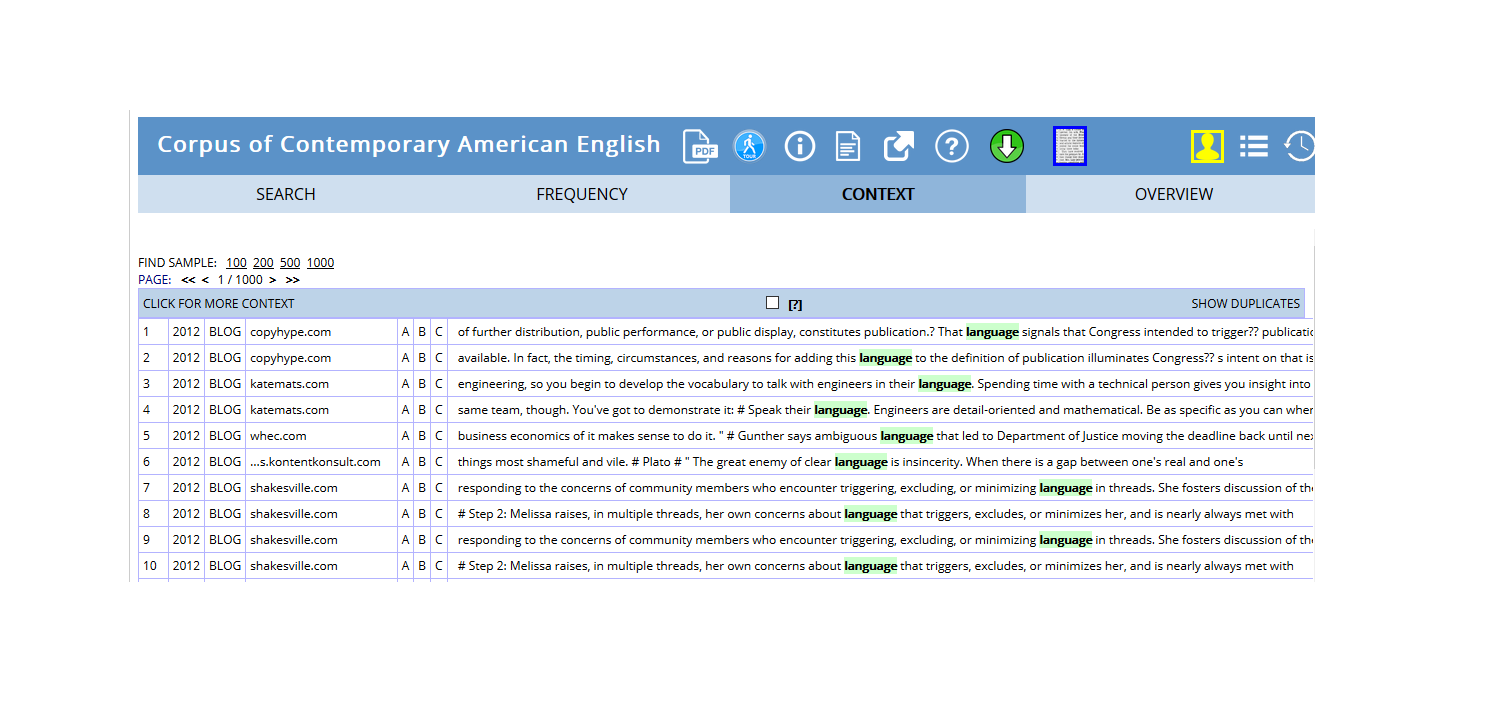{ width=100% } #### Lextutor and Other Web Concordancers [Lextutor](https://www.lextutor.ca/) offers free web-based tools including concordancers, vocabulary profilers, and more. **When to use web concordancers:** - Classroom demonstrations (no installation) - Quick vocabulary lookups - Exploring concordancing concepts - Public/shared computers - Mobile devices ### Programming-Based Solutions {#programming} For maximum flexibility, reproducibility, and integration with other analytical tools, programming languages offer unmatched power. #### R with quanteda (Our Focus) **Why R and quanteda for concordancing:** **Reproducibility:** - Scripts document every step - Share exact methodology with colleagues - Regenerate results precisely - Satisfy open science requirements - Version control with Git **Flexibility:** - Custom search patterns - Unlimited filtering and grouping - Integration with data manipulation (dplyr) - Combine concordancing with statistics - Automated workflows for large projects **Integration:** - Connect to databases - Web scraping for corpus building - Statistical modeling on results - Machine learning pipelines - Advanced visualization (ggplot2) **Scalability:** - Handle massive datasets - Parallel processing for speed - Cloud computing integration - Automated batch processing - Memory-efficient for large corpora **Cost:** - Completely free and open source - No licensing fees ever - Extensive package ecosystem - Active development community **When to use R/quanteda:** - Reproducible research publications - Complex analytical workflows - Large-scale or custom corpora - Integration with statistics/modeling - Automated/repeating analyses - When you need to document everything **Learning investment:** - Steeper initial learning curve than GUI tools - Programming basics required - But: transferable skills across research career - Worth it for serious corpus work - This tutorial will guide you! #### Python with NLTK and Others Python offers similar advantages through packages like NLTK, spaCy, and others. **When Python might be better:** - You already know Python - Heavy NLP preprocessing needed - Machine learning focus - Web development integration - You're in a Python-centric community **For most linguistic concordancing, R/quanteda is excellent.** #### Our Interactive Notebook Tool The [Concordancing Tool](https://binderhub.atap-binder.cloud.edu.au/v2/gh/SLCLADAL/interactive-notebooks-environment/main?urlpath=git-pull%3Frepo=https://github.com/SLCLADAL/interactive-notebooks%26urlpath=lab/tree/interactive-notebooks/notebooks/kwictool.ipynb%26branch=main) bridges GUI and programming approaches: **Features:** - Upload your own texts - Pre-written code chunks (just click run) - Modify code as you learn - Download results (CSV, Excel) - No installation needed - Reproducible but accessible **When to use:** - Learning concordancing and coding together - One-off analyses - Quick results with your own texts - Sharing with non-programmers - Teaching hybrid approaches ## Choosing the Right Tool {#choosing-tool} Different tasks call for different tools. Many researchers use multiple approaches: | Task | Recommended Tool | Why | |------|------------------|-----| | Teaching basics | AntConc or Web interfaces | Zero barrier to entry, visual, immediate | | Quick exploration | Web corpora (COCA, etc.) | No setup, instant results | | Translation work | ParaConc or SketchEngine | Purpose-built for parallel texts | | Publication research | WordSmith or R | Professional features, reproducibility | | Large custom corpora | R/Python | Scalability, automation | | Reproducible workflows | R/Python | Script everything, version control | | Team projects | SketchEngine or R | Collaboration features | | Learning to code | Our notebook tool | Gentle introduction | **Pro tip:** Start with AntConc or web interfaces to learn concepts, then graduate to R when you need more power or reproducibility. ## Why Use R for Concordancing? {#why-r} Given the excellent GUI tools available, why invest in learning R for concordancing? ### The Reproducibility Imperative Modern science increasingly demands reproducibility: **With GUI tools:** - "I opened AntConc, loaded corpus X, searched for Y, sorted by..." - Hard to document exact steps - Difficult for others to replicate - Easy to forget what you did **With R scripts:** ```r # Load corpus corpus <-readLines("my_texts.txt") # Create concordance kwic_result <- quanteda::kwic( tokens(corpus), pattern ="test_pattern", window =5) # Filter and arrange kwic_filtered <- kwic_result |>filter(str_detect(post, "specific_pattern")) |>arrange(pre) # Export write.csv(kwic_filtered, "results.csv") ```- Every step explicit - Exact replication possible - Share script with paper - Satisfies open science standards ### Integration and Power **Seamless workflow:** ```r # 1. Build corpus texts <-scrape_websites(urls) # 2. Concordance kwics <-kwic(tokens(texts), pattern) # 3. Statistical analysis collocation_test(kwics) # 4. Visualization ggplot(kwics) + ... # 5. Modeling regression_model <-lm(frequency ~ variables) # All in one environment! ```**vs. GUI approach:** - Export from concordancer - Import to Excel - Clean/rearrange - Import to statistics software - Export results - Import to visualization tool - Hope nothing was lost in translation! ### Customization and Control **R allows:** - Custom search patterns beyond tool limitations - Arbitrary filtering logic - Novel analysis approaches - Integration with your specific workflow - Automation of repetitive tasks - Handling of unusual data formats **Example: Complex filtering** ```r # Find "must" but only: # - In questions # - Followed by a verb # - Not in negation # - In formal register # Easy in R, impossible/tedious in GUI tools ```### Scalability **GUI tools struggle with:** - Thousands of text files - Gigabyte+ corpora - Batch processing - Complex workflows - Memory limitations **R handles:** - Massive datasets efficiently - Parallel processing - Cloud computing - Automated pipelines - Memory management ### The Learning Investment **Yes, R has a learning curve.** But: - Skills transfer across research career - Massive online community - Extensive free resources - Used across disciplines - Increasingly expected in academia - This tutorial guides you step-by-step! **You don't need to be a programmer** - basic R suffices for concordancing, and you'll learn by doing. ### When GUI Tools Are Better **Use GUI tools when:** - Quick one-off exploration - Teaching complete beginners - Working with non-technical collaborators - You need results immediately - The analysis is truly simple - Learning R isn't worth it for this project **But consider R when:** - Doing serious research - Need reproducibility - Complex or custom analysis - Working with large corpora - Building a research program - Want transferable skills ### Exercise 2.1: Tool Comparison {.exercise} ::: {.callout-warning icon=false} ## Hands-On Tool Exploration **Task:** Search for the same pattern in the same text using two different tools. 1. Choose a simple text (e.g., a news article) 2. Search for a word (e.g., "government") 3. Try in: - AntConc (download and use) - A web concordancer (e.g., Lextutor) - OR our R notebook tool **Compare:** - Which was easiest to set up? - Which gave you most control? - Which had best export options? - Which would you use for what purposes? **Discuss:** - What are the trade-offs? - When would each be appropriate? - What features matter most to you? ::: --- # Part 3: Getting Started with R Concordancing {#part3} Now we'll move from theory to practice, learning to create concordances using R and the quanteda package. ## Setup and Installation {#setup} ### Installing Required Packages If you're new to R, see our [Getting Started with R](/tutorials/intror/intror.html) tutorial first. **Install packages (run once):** ```{r prep1, echo=T, eval = F} # Install core packages install.packages("quanteda") # Text analysis framework install.packages("dplyr") # Data manipulation install.packages("stringr") # String processing install.packages("writexl") # Excel export install.packages("here") # File path management install.packages("flextable") # Pretty tables install.packages("tidyr") # Data reshaping ```This may take a few minutes. Don't worry if you see red text—that's normal installation output, not necessarily errors! ### Loading Packages **Load packages (run every session):** ```{r prep2, message=FALSE, warning=FALSE, class.source='klippy'} # Load packages library(quanteda) # Core concordancing library(dplyr) # Data wrangling library(stringr) # String manipulation library(writexl) # Export to Excel library(here) # Smart file paths library(flextable) # Display tables library(tidyr) # Reshape data ```::: {.callout-tip} ## Package Loading Best Practice **Always load packages at the top of your script** Benefits: - Clear what dependencies you have - Others can see what they need to install - Easier to troubleshoot if something's missing - Professional script organization ```r # Good practice library(quanteda) library(dplyr) # ... rest of script # Poor practice # Code scattered throughout library(quanteda) # more code library(dplyr) # forgot earlier # more code ```::: ## Loading Your First Text {#loading-text} We'll use Lewis Carroll's *Alice's Adventures in Wonderland* as our example text. This classic provides: - Rich literary language - Memorable characters and phrases - Sufficient length for meaningful patterns - Public domain (freely available) ### Loading from Project Gutenberg Project Gutenberg provides free access to thousands of public domain texts. ```{r skwic2, warning=F, message=F} # Load Alice's Adventures in Wonderland rawtext <- readLines("https://www.gutenberg.org/files/11/11-0.txt") ``````{r skwic2b, echo=FALSE, message=FALSE, warning=FALSE, class.source='klippy'} # Inspect first 25 non-empty lines rawtext |> as.data.frame() |> dplyr::filter(rawtext != "") |> head(25) |> flextable::flextable() |> flextable::set_table_properties(width = .95, layout = "autofit") |> flextable::theme_zebra() |> flextable::fontsize(size = 12) |> flextable::fontsize(size = 12, part = "header") |> flextable::align_text_col(align = "center") |> flextable::set_caption(caption = "First 25 non-empty lines of Alice's Adventures in Wonderland from Project Gutenberg.") |> flextable::border_outer() ```**What just happened:** - `readLines()` fetched the text file from the web - Each line became an element in a vector called `rawtext`- We now have the complete book in R memory ### Understanding the Raw Text Structure Looking at the output, we see: - **Line 1-30**: Title page, legal information, contents - **Real text starts**: After "CHAPTER I" - **Formatting**: Chapter headings, line breaks, spaces This is typical of Project Gutenberg texts—they include metadata and formatting we need to handle. ## Data Preparation: Cleaning the Text {#cleaning} Raw texts require preprocessing before analysis. This crucial step ensures clean, analysis-ready data. ### Why Data Preparation Matters **The reality of text data:** - Downloaded texts include metadata (titles, licenses, etc.) - Formatting varies (line breaks, spaces, special characters) - Inconsistencies abound (encodings, punctuation) - Structure needs standardization **Impact on analysis:** - Bad: Metadata contaminates results - Bad: Formatting breaks pattern matching - Bad: Inconsistencies cause missed matches - Good: Clean data = reliable results ::: {.callout-important} ## The 80/20 Rule of Text Analysis Researchers often spend: - **80% of time**: Cleaning and preparing data - **20% of time**: Actually analyzing it This isn't wasted time—it's **essential investment**. Poor preparation leads to unreliable results, wasted effort, and potentially wrong conclusions. **The payoff:** - Accurate results - Reproducible analyses - Confidence in findings - Time saved troubleshooting later ::: ### Cleaning Alice in Wonderland Let's transform our raw text into analysis-ready format: ```{r skwic3, message=F, warning=F} text <- rawtext |> # Collapse all lines into one continuous text paste0(collapse = " ") |> # Remove extra white spaces (multiple spaces → single space) stringr::str_squish() |> # Remove everything before "CHAPTER I." (title page, contents, etc.) stringr::str_remove(".*CHAPTER I\\.") ``````{r skwic3b, echo = F, message=FALSE, warning=FALSE} # Display first 1000 characters text |> substr(start = 1, stop = 1000) |> as.data.frame() |> flextable() |> flextable::set_table_properties(width = .95, layout = "autofit") |> flextable::theme_zebra() |> flextable::fontsize(size = 12) |> flextable::fontsize(size = 12, part = "header") |> flextable::align_text_col(align = "center") |> flextable::set_caption(caption = "First 1000 characters of cleaned Alice text—ready for concordancing!") |> flextable::border_outer() ```**What each step does:** **1. `paste0(collapse = " ")`** - Joins all separate lines into one continuous string - Why: Concordancing works better on continuous text - Prevents artificial line-break effects on patterns **2. `stringr::str_squish()`** - Removes leading/trailing whitespace - Reduces multiple spaces to single space - Standardizes spacing throughout **3. `stringr::str_remove(".*CHAPTER I\\.")`** - Removes everything up to and including "CHAPTER I." - `.*` means "any characters" - `\\.` means a literal period (escaped) - Isolates the actual story text ::: {.callout-note} ## Understanding the Regular Expression The pattern `".*CHAPTER I\\."` breaks down as: - `.` = any character - `*` = zero or more times - `CHAPTER I` = literal text - `\\.` = escaped period (`.` is special in regex) **Together**: "Match any amount of any characters, followed by 'CHAPTER I.'" Regular expressions are powerful pattern-matching tools we'll explore more later! ::: ### Exercise 3.1: Text Preparation Practice {.exercise} ::: {.callout-warning icon=false} ## Clean Your Own Text **Load a different Project Gutenberg text:** ```{r ex3_1_setup, eval=FALSE} # Example: Pride and Prejudice raw_pride <- readLines("https://www.gutenberg.org/files/1342/1342-0.txt") ```**Your tasks:** 1. Examine the first 50 lines—what needs removing? 2. Find where the actual text starts (look for "Chapter" or similar) 3. Clean the text using the Alice example as a model 4. Verify your result looks correct **Questions:** - What patterns did you use to identify the start of the text? - Were there any challenges specific to this text? - How would you generalize this cleaning procedure? **Bonus:** Write a function that automates Gutenberg text cleaning: ```{r ex3_1_bonus, eval=FALSE} clean_gutenberg <- function(url, start_pattern) { # Your code here } ```::: --- # Part 4: Creating Your First Concordance {#part4} Now that we have clean text, let's extract our first concordances! ## Basic KWIC Extraction {#basic-kwic} The `kwic()` function from quanteda makes concordancing straightforward. ### Your First Concordance Let's search for "Alice": ```{r basekwic2, message=F, warning=F} mykwic <- quanteda::kwic( quanteda::tokens(text), # Tokenize the text first pattern = quanteda::phrase("Alice")) |> # What to search for as.data.frame() # Convert to data frame ``````{r basekwic2b, echo=FALSE, message=FALSE, warning=FALSE, class.source='klippy'} # Display first 6 concordance lines mykwic |> head() |> flextable::flextable() |> flextable::set_table_properties(width = .95, layout = "autofit") |> flextable::theme_zebra() |> flextable::fontsize(size = 12) |> flextable::fontsize(size = 12, part = "header") |> flextable::align_text_col(align = "center") |> flextable::set_caption(caption = "First 6 concordance lines for 'Alice' in our example text.") |> flextable::border_outer() ```**Success!** You've created your first concordance. Let's understand what happened. ### Understanding the `kwic()` Function **Function structure:** ```r kwic( x =, # The tokenized text pattern =, # What to search for window =, # Context size (default: 5) ... # Other options ) ```**Required arguments:** - `x`: Must be a **tokens object** (created by `tokens()`) - `pattern`: What you're searching for **Important pattern specification:** - `quanteda::phrase("Alice")` = exact phrase (case-sensitive) - Without `phrase()`, searches for individual tokens - We'll explore more pattern types soon! ### The Concordance Table Structure The result is a data frame with these columns: | Column | Contains | Purpose | |--------|----------|---------| | `docname` | Document name | Track source (useful for multi-text corpora) | | `from` | Start position | Where match begins (token number) | | `to` | End position | Where match ends | | `pre` | Left context | Words before the keyword | | `keyword` | The match | Your search term | | `post` | Right context | Words after the keyword | | `pattern` | Search pattern | What you searched for (useful when searching multiple patterns) | ### Exploring Your Concordance **How many matches did we find?** ```{r basekwic4} nrow(mykwic) # Count rows ```OR ```{r basekwic5} length(mykwic$keyword) # Count keywords ```We found `r nrow(mykwic)` instances of "Alice" in the text! **What variations were found?** ```{r basekwic6} table(mykwic$keyword) ```All instances are exactly "Alice" (case-sensitive match). ### Adjusting the Context Window The default context is 5 words on each side. Sometimes you need more: ```{r basekwic8, message=F, warning=F} mykwic_long <- quanteda::kwic( quanteda::tokens(text), pattern = quanteda::phrase("alice"), window = 10) |> # Extended context! as.data.frame() ``````{r skwic8b, echo=FALSE, message=FALSE, warning=FALSE, class.source='klippy'} # Display with longer context mykwic_long |> head() |> flextable::flextable() |> flextable::set_table_properties(width = .95, layout = "autofit") |> flextable::theme_zebra() |> flextable::fontsize(size = 12) |> flextable::fontsize(size = 12, part = "header") |> flextable::align_text_col(align = "center") |> flextable::set_caption(caption = "Concordances with extended 10-word context windows.") |> flextable::border_outer() ```**When to use wider windows:** - Understanding full sentence context - Analyzing longer constructions - Studying distant relationships - Literary analysis requiring more text **When to use narrower windows:** - Focused on immediate collocates - Large result sets (easier to scan) - Identifying local patterns - Quick exploration ::: {.callout-tip} ## Choosing Context Window Size **General guidelines:** - **5 words** (default): Good starting point for most analyses - **3 words**: Immediate collocates, tight focus - **10-15 words**: Sentence-level context - **20+ words**: Paragraph-level context (rare, usually too much) **Experiment!** Try different sizes and see what reveals patterns best for your research question. ::: ### Exercise 4.1: Basic Concordancing Practice {.exercise} ::: {.callout-warning icon=false} ## Your Turn! Using the Alice text, complete these tasks: **1. Extract concordances for "confused"** <details> <summary>Answer</summary> ```{r ex4_1_1, class.source = NULL, eval = T} kwic_confused <- quanteda::kwic( x = quanteda::tokens(text), pattern = quanteda::phrase("confused") ) # Display first 10 kwic_confused |> as.data.frame() |> head(10) ```</details> **2. How many times does "wondering" appear?** <details> <summary>Answer</summary> ```{r ex4_1_2, class.source = NULL, eval = T} quanteda::kwic( x = quanteda::tokens(text), pattern = quanteda::phrase("wondering") ) |> as.data.frame() |> nrow() ```There are `r nrow(quanteda::kwic(x = quanteda::tokens(text), pattern = quanteda::phrase("wondering")))` instances. </details> **3. Extract "strange" with a 7-word window, show first 5 lines** <details> <summary>Answer</summary> ```{r ex4_1_3, class.source = NULL, eval = T} kwic_strange <- quanteda::kwic( x = quanteda::tokens(text), pattern = quanteda::phrase("strange"), window = 7 ) kwic_strange |> as.data.frame() |> head(5) ```</details> **Challenge:** Pick your own word and explore different window sizes. Which size reveals the most about how the word is used? ::: --- # Part 5: Exporting and Saving Concordances {#part5} Once you've created concordances, you'll often want to save them for further analysis, sharing, or documentation. ## Exporting to Excel {#export-excel} Excel spreadsheets are widely compatible and easy to share with colleagues. ```{r export_demo, eval=F, warning=F, message=F} # Export to Excel write_xlsx(mykwic, here::here("my_alice_concordance.xlsx")) ```**What this does:** - `write_xlsx()` creates an Excel file (.xlsx) - `here::here()` saves it in your working directory - Result: A spreadsheet with all concordance data ::: {.callout-tip} ## Using `here()` for File Paths The `here` package makes file paths easier and more portable: ```{r here_demo, eval=FALSE} # Without here - breaks if you move project write_xlsx(data, "C:/Users/YourName/Documents/project/file.xlsx") # With here - works anywhere write_xlsx(data, here::here("file.xlsx")) # Subdirectories write_xlsx(data, here::here("output", "results", "file.xlsx")) ```**Benefits:** - Works on Windows, Mac, Linux - No hard-coded paths - Project-relative paths - Collaborators can run your code ::: ## Other Export Formats {#other-exports} ```{r other_exports, eval=FALSE} # CSV (universal, simple) write.csv(mykwic, here::here("concordance.csv"), row.names = FALSE) # Tab-separated (good for large texts) write.table(mykwic, here::here("concordance.txt"), sep = "\t", row.names = FALSE) # R data format (preserves all R attributes) saveRDS(mykwic, here::here("concordance.rds")) # Load RDS back later mykwic_loaded <- readRDS(here::here("concordance.rds")) ```**When to use each:** | Format | Best For | Why | |--------|----------|-----| | Excel (.xlsx) | Sharing with non-R users | Widely compatible, can open directly | | CSV | Simple data exchange | Universal, plain text, version control friendly | | TSV/TXT | Very large datasets | Smaller file size than Excel | | RDS | R-to-R sharing | Preserves all object attributes, efficient | ## Creating Export-Ready Tables {#export-tables} For presentations or reports, format your concordances nicely: ```{r export_table, eval=FALSE} # Create a nicely formatted subset mykwic |> head(20) |> # First 20 for manageable size select(pre, keyword, post) |> # Just the interesting columns flextable() |> set_caption("Concordance of 'Alice' in Alice's Adventures in Wonderland") |> theme_zebra() |> autofit() |> save_as_docx(path = here::here("concordance_table.docx")) ```This creates a Word document with a professional-looking table—perfect for embedding in papers! # Part 6: Advanced Pattern Matching {#part6} ## Multi-Word Expressions and Phrases {#multiword} While single words are common search targets, language research often requires extracting phrases or multi-word expressions (MWEs). ### Why Multi-Word Expressions Matter **Language is more than individual words:** - Idioms: "kick the bucket", "spill the beans" - Collocations: "strong coffee", "make a decision" - Fixed expressions: "by and large", "as a matter of fact" - Titles and names: "Mad Hatter", "Cheshire Cat" - Technical terms: "global warming", "machine learning" These MWEs often function as single semantic units despite containing multiple words. Searching for individual words misses the unified meaning. ### Extracting Phrases with quanteda The `phrase()` function tells quanteda to treat multiple words as a single search unit: ```{r multikwic2, message=FALSE, warning=FALSE} # Search for "poor alice" as a phrase kwic_pooralice <- quanteda::kwic( quanteda::tokens(text), pattern = quanteda::phrase("poor alice")) |> as.data.frame() ``````{r multikwic2b, echo=FALSE, message=FALSE, warning=FALSE, class.source='klippy'} # Display results kwic_pooralice |> head(10) |> flextable::flextable() |> flextable::set_table_properties(width = .95, layout = "autofit") |> flextable::theme_zebra() |> flextable::fontsize(size = 12) |> flextable::fontsize(size = 12, part = "header") |> flextable::align_text_col(align = "center") |> flextable::set_caption(caption = "Concordances for the phrase 'poor alice' in Alice's Adventures in Wonderland.") |> flextable::border_outer() ```**What `phrase()` does:** - Treats "poor alice" as an inseparable unit - Both words must appear consecutively - Respects word boundaries - Case-sensitive by default **Without `phrase()`:** ```{r no_phrase_demo, eval=FALSE} # This would match "poor" and "alice" separately, anywhere in the text kwic(tokens(text), pattern = c("poor", "alice")) ```### Case Sensitivity Control By default, searches are case-sensitive. Control this behavior: ```{r case_demo, eval=FALSE} # Case-sensitive (default) - only matches exactly "Alice" kwic(tokens(text), pattern = quanteda::phrase("Alice")) # Case-insensitive - matches "Alice", "alice", "ALICE", etc. kwic(tokens(text, remove_punct = TRUE), pattern = quanteda::phrase("alice"), case_insensitive = TRUE) ```::: {.callout-tip} ## When to Use Case-Insensitive Search **Use case-insensitive when:** - Names might be capitalized variably - Sentence-initial position matters - Historical texts with inconsistent capitalization - You want all variants regardless of position **Keep case-sensitive when:** - Proper names vs. common words matter (e.g., "Apple" vs. "apple") - You're studying capitalization patterns - Precision is more important than recall ::: ### Searching Multiple Phrases Search for several phrases simultaneously: ```{r multiple_phrases, eval=FALSE} # Search for multiple character descriptions patterns <- c("poor alice", "little alice", "dear alice") kwic_alice_variants <- quanteda::kwic( quanteda::tokens(text), pattern = phrase(patterns) ) |> as.data.frame() # See which variants were found table(kwic_alice_variants$keyword) ```### Exercise 6.1: Phrase Extraction {.exercise} ::: {.callout-warning icon=false} ## Practice with Phrases **1. Extract "the hatter" (first 10 lines)** <details> <summary>Answer</summary> ```{r ex6_1_1, eval=T} kwic_thehatter <- quanteda::kwic( x = quanteda::tokens(text), pattern = quanteda::phrase("the hatter") ) kwic_thehatter |> as.data.frame() |> head(10) ```</details> **2. How many instances of "the hatter"?** <details> <summary>Answer</summary> ```{r ex6_1_2, eval=T} kwic_thehatter |> as.data.frame() |> nrow() ```There are `r nrow(kwic_thehatter)` instances. </details> **3. Extract "the cat" (first 5 lines)** <details> <summary>Answer</summary> ```{r ex6_1_3, eval=T} kwic_thecat <- quanteda::kwic( x = quanteda::tokens(text), pattern = quanteda::phrase("the cat") ) kwic_thecat |> as.data.frame() |> head(5) ```</details> **Challenge:** Find all instances of character names with titles (e.g., "the Duchess", "the King", "the Queen"). How would you search for these patterns efficiently? ::: --- # Part 7: Regular Expressions for Power Users {#part7} Regular expressions (regex) provide powerful pattern-matching capabilities beyond exact words or phrases. ## Understanding Regular Expressions {#regex-intro} A **regular expression** is a sequence of characters that describes a search pattern. Think of it as a wildcard on steroids. ### Why Regular Expressions Matter **Without regex:** - Search for "walk", "walks", "walked", "walking" separately - Four searches, combine results manually - Miss any variants you didn't think of **With regex:** - `"walk.*"` finds all forms in one search - Captures "walks", "walked", "walking", "walker", etc. - Systematic, comprehensive ### Regular Expression Types There are three fundamental categories: #### 1. Symbols for Frequencies These control how many times a pattern appears: ```{r regex_freq_table, echo=FALSE, eval=T, message=FALSE, warning=FALSE} symbols1 <- c("?", "*", "+", "{n}", "{n,}", "{n,m}") explanation1 <- c( "Preceding item is optional (0 or 1 times)", "Preceding item appears 0 or more times", "Preceding item appears 1 or more times", "Preceding item appears exactly n times", "Preceding item appears n or more times", "Preceding item appears n to m times" ) example1 <- c( "walk[a-z]? → walk, walks", "walk[a-z]* → walk, walks, walked, walking", "walk[a-z]+ → walks, walked, walking (not walk)", "walk[a-z]{2} → walked", "walk[a-z]{2,} → walked, walking", "walk[a-z]{2,3} → walked, walking" ) data.frame(Symbol = symbols1, Explanation = explanation1, Example = example1) |> flextable::flextable() |> flextable::set_table_properties(width = .95, layout = "autofit") |> flextable::theme_zebra() |> flextable::fontsize(size = 12) |> flextable::fontsize(size = 12, part = "header") |> flextable::set_caption(caption = "Regular expression symbols for frequency matching.") |> flextable::border_outer() ```#### 2. Character Classes These represent groups of characters: ```{r regex_classes_table, echo=FALSE, eval=T, message=FALSE, warning=FALSE} symbols2 <- c( "[ab]", "[AB]", "[12]", "[:digit:]", "[:lower:]", "[:upper:]", "[:alpha:]", "[:alnum:]", "[:punct:]", "[:space:]", "." ) explanations2 <- c( "Lowercase a or b", "Uppercase A or B", "Digits 1 or 2", "Any digit: 0-9", "Any lowercase letter: a-z", "Any uppercase letter: A-Z", "Any letter: a-z, A-Z", "Any letter or digit", "Any punctuation character", "Any whitespace (space, tab, newline)", "Any single character (wildcard)" ) data.frame(Symbol = symbols2, Explanation = explanations2) |> flextable::flextable() |> flextable::set_table_properties(width = .75, layout = "autofit") |> flextable::theme_zebra() |> flextable::fontsize(size = 12) |> flextable::fontsize(size = 12, part = "header") |> flextable::set_caption(caption = "Regular expression character classes.") |> flextable::border_outer() ```#### 3. Position Anchors These specify where patterns must appear: ```{r regex_anchors_table, echo=FALSE, eval=T, message=FALSE, warning=FALSE} symbols3 <- c("\\\\b", "\\\\B", "^", "$", "<", ">") explanations3 <- c( "Word boundary (start or end of word)", "Not a word boundary (inside a word)", "Start of string/line", "End of string/line", "Start of word", "End of word" ) data.frame(Symbol = symbols3, Explanation = explanations3) |> flextable::flextable() |> flextable::set_table_properties(width = .6, layout = "autofit") |> flextable::theme_zebra() |> flextable::fontsize(size = 12) |> flextable::fontsize(size = 12, part = "header") |> flextable::set_caption(caption = "Regular expression position anchors.") |> flextable::border_outer() ```## Using Regular Expressions in Concordancing {#regex-kwic} To use regex in `kwic()`, set `valuetype = "regex"`: ```{r rkwic6, message=FALSE, warning=FALSE} # Find words starting with "alic" OR "hatt" patterns <- "\\b(alic|hatt).*" kwic_regex <- quanteda::kwic( quanteda::tokens(text), pattern = patterns, valuetype = "regex") |> as.data.frame() ``````{r rkwic6b, echo=FALSE, message=FALSE, warning=FALSE, class.source='klippy'} kwic_regex |> head(10) |> flextable::flextable() |> flextable::set_table_properties(width = .95, layout = "autofit") |> flextable::theme_zebra() |> flextable::fontsize(size = 12) |> flextable::fontsize(size = 12, part = "header") |> flextable::align_text_col(align = "center") |> flextable::set_caption(caption = "Concordances using regex pattern to find words beginning with 'alic' or 'hatt'.") |> flextable::border_outer() ```**Pattern breakdown:** - `\\b` = word boundary (start of word) - `(alic|hatt)` = either "alic" OR "hatt" - `.*` = followed by any characters - Result: "alice", "hatter", "hatters" but NOT "malice" or "shatter" ### Common Regex Patterns for Concordancing **Find all forms of a word:** ```{r regex_patterns, eval=FALSE} # All forms of "think" kwic(tokens(text), pattern = "\\bthink.*", valuetype = "regex") # Matches: think, thinks, thinking, thought, thinker # Words ending in "ing" kwic(tokens(text), pattern = ".*ing\\b", valuetype = "regex") # Words ending in "tion" kwic(tokens(text), pattern = ".*tion\\b", valuetype = "regex") ```**Find words of specific length:** ```{r length_patterns, eval=FALSE} # Three-letter words kwic(tokens(text), pattern = "\\b[a-z]{3}\\b", valuetype = "regex") # Words 10+ letters long kwic(tokens(text), pattern = "\\b[a-z]{10,}\\b", valuetype = "regex") ```**Find patterns with specific structure:** ```{r structure_patterns, eval=FALSE} # Words with double letters kwic(tokens(text), pattern = "\\b\\w*(.)\\1\\w*\\b", valuetype = "regex") # Matches: little, bottle, matters, etc. # Words starting with vowels kwic(tokens(text), pattern = "\\b[aeiou]\\w*", valuetype = "regex") ```::: {.callout-warning} ## Regex Can Be Tricky! Regular expressions are powerful but can be: - **Cryptic**: `\\b(?:alic|hatt).*` looks like gibberish at first - **Fragile**: Small changes can break patterns - **Surprising**: They might match more (or less) than you expect **Best practices:** - Test patterns on small samples first - Use online regex testers (regex101.com) - Comment your patterns explaining what they do - Start simple, add complexity gradually - Check results carefully—regex can surprise you! ::: ### Exercise 7.1: Regular Expression Practice {.exercise} ::: {.callout-warning icon=false} ## Mastering Regex **1. Find words containing "exu" (first 10)** <details> <summary>Answer</summary> ```{r ex7_1_1, eval=T} kwic_exu <- quanteda::kwic( x = quanteda::tokens(text), pattern = ".*exu.*", valuetype = "regex" ) kwic_exu |> as.data.frame() |> head(10) ```</details> **2. How many words begin with "pit"?** <details> <summary>Answer</summary> ```{r ex7_1_2, eval=T} quanteda::kwic( x = quanteda::tokens(text), pattern = "\\bpit.*", valuetype = "regex" ) |> as.data.frame() |> nrow() ```</details> **3. Find words ending in "ption" (first 5)** <details> <summary>Answer</summary> ```{r ex7_1_3, eval=T} quanteda::kwic( x = quanteda::tokens(text), pattern = ".*ption\\b", valuetype = "regex" ) |> as.data.frame() |> head(5) ```</details> **Challenge:** 1. Find all words starting with "un-" (negative prefix) 2. Find all words with exactly 4 letters 3. Find all words containing "qu" 4. Find words that appear to be capitalized names (hint: uppercase start) ::: --- # Part 8: Filtering and Refining Concordances {#part8} Raw concordances are just the starting point. The real power comes from filtering, sorting, and refining results to reveal patterns. ## Piping for Conditional Concordances {#piping} Often we want concordances only when specific conditions are met. **Piping** with dplyr makes this elegant. ### The Pipe Operator: `|>` or `%>%` Piping chains operations together: "do this, **then** do that" ```{r pipe_concept, eval=FALSE} # Without piping (nested, hard to read) filter(as.data.frame(kwic(tokens(text), "alice")), condition) # With piping (clear, sequential) kwic(tokens(text), "alice") |> as.data.frame() |> filter(condition) # Read as: "take text, make concordance, convert to dataframe, filter" ```### Filtering by Context Find "alice" only when preceded by "poor" or "little": ```{r pipekwic7, echo=T, eval=T, message=FALSE, warning=FALSE} quanteda::kwic( x = quanteda::tokens(text), pattern = "alice") |> as.data.frame() |> # Filter: "pre" column must end with "poor" or "little" dplyr::filter(stringr::str_detect(pre, "poor$|little$")) -> kwic_pipe ``````{r pipekwic7b, echo=FALSE, message=FALSE, warning=FALSE, class.source='klippy'} kwic_pipe |> head(10) |> flextable::flextable() |> flextable::set_table_properties(width = .95, layout = "autofit") |> flextable::theme_zebra() |> flextable::fontsize(size = 12) |> flextable::fontsize(size = 12, part = "header") |> flextable::align_text_col(align = "center") |> flextable::set_caption(caption = "Instances of 'alice' preceded by 'poor' or 'little'.") |> flextable::border_outer() ```**Pattern breakdown:** - `str_detect(pre, "poor$|little$")`- Check if `pre` (preceding context) contains... - `poor$` = "poor" at the end ($ = end anchor) - `|` = OR - `little$` = "little" at the end **Why the `$` matters:** - `"poor$"` = must be last word before keyword - `"poor"` = anywhere in preceding context - Precision prevents false matches like "poorly alice" ### Multiple Conditions Combine filters for complex queries: ```{r complex_filter, eval=FALSE} kwic(tokens(text), "said") |> as.data.frame() |> # Must be preceded by name AND followed by specific punctuation filter( str_detect(pre, "Alice$|Hatter$|Queen$"), str_detect(post, "^,|^\\.") ) ```This finds speech acts: "[Character] said, ..." ### Filtering by Position Find instances only at specific positions in the text: ```{r position_filter, eval=FALSE} kwic(tokens(text), "alice") |> as.data.frame() |> # Only in first 1000 tokens filter(from <= 1000) # Only in last quarter of text max_position <- max(from) kwic_data |> filter(from >= max_position * 0.75) ```## Sorting and Arranging Concordances {#sorting} Reordering concordances reveals patterns invisible in occurrence order. ### Alphabetical Sorting Sort by what follows the keyword: ```{r orderkwic2, echo=T, eval=T, message=FALSE, warning=FALSE} quanteda::kwic( x = quanteda::tokens(text), pattern = "alice") |> as.data.frame() |> # Arrange alphabetically by following context dplyr::arrange(post) -> kwic_ordered ``````{r orderkwic2b, echo=FALSE, message=FALSE, warning=FALSE, class.source='klippy'} kwic_ordered |> head(10) |> flextable::flextable() |> flextable::set_table_properties(width = .95, layout = "autofit") |> flextable::theme_zebra() |> flextable::fontsize(size = 12) |> flextable::fontsize(size = 12, part = "header") |> flextable::align_text_col(align = "center") |> flextable::set_caption(caption = "Concordances sorted alphabetically by following word.") |> flextable::border_outer() ```**Why sort alphabetically?** - Groups similar contexts together - Reveals collocational patterns - Makes manual analysis easier - Identifies semantic prosody **Sort by different columns:** ```{r sort_variations, eval=FALSE} arrange(pre) # By preceding context arrange(keyword) # By matched pattern (if searching multiple) arrange(from) # By position in text (chronological) ```### Sorting by Frequency More powerful: arrange by how common collocates are. #### Step-by-Step Frequency Sorting ```{r arrange_kwic, echo=T, eval=T, message=FALSE, warning=FALSE} quanteda::kwic( x = quanteda::tokens(text), pattern = "alice" ) |> as.data.frame() |> # Extract first word after keyword dplyr::mutate(post1 = str_remove_all(post, " .*")) |> # Group by that word dplyr::group_by(post1) |> # Count frequency of each dplyr::mutate(post1_freq = n()) |> # Sort by frequency (descending) dplyr::arrange(-post1_freq) -> kwic_ordered_coll ``````{r orderkwic4j, echo=FALSE, message=FALSE, warning=FALSE, class.source='klippy'} kwic_ordered_coll |> head(10) |> flextable::flextable() |> flextable::set_table_properties(width = .95, layout = "autofit") |> flextable::theme_zebra() |> flextable::fontsize(size = 12) |> flextable::fontsize(size = 12, part = "header") |> flextable::align_text_col(align = "center") |> flextable::set_caption(caption = "Concordances sorted by frequency of following word.") |> flextable::border_outer() ```**What each step does:** 1. **`mutate(post1 = str_remove_all(post, " .*"))`** - Creates new column `post1` - Extracts just the first word after keyword - Removes everything after first space 2. **`group_by(post1)`** - Groups all rows with same following word - Enables per-group calculations 3. **`mutate(post1_freq = n())`** - Counts how many in each group - `n()` returns group size - Adds frequency to each row 4. **`arrange(-post1_freq)`** - Sorts by frequency - `-` means descending (highest first) - Most common collocates appear first **Why frequency sorting matters:** - Reveals strongest collocational patterns - Identifies typical vs. unusual usage - Quantifies intuitions - Prioritizes analysis (examine common patterns first) ### Multi-Level Sorting Sort by multiple criteria: ```{r multilevel_sort, eval=FALSE} kwic_data |> arrange(-post1_freq, -post2_freq, pre1) # Read as: "sort by post1 frequency (desc), # then post2 frequency (desc), # then pre1 (ascending)" ```## Extracting N-grams Around Keywords {#ngrams} Sometimes you want to analyze not just the next word, but the next 2-3 words (bigrams, trigrams). ```{r ngrams_demo, eval=FALSE} mykwic |> rowwise() |> mutate( # First word after post1 = unlist(strsplit(post, " "))[1], # Second word after post2 = unlist(strsplit(post, " "))[2], # Third word after post3 = unlist(strsplit(post, " "))[3], # Last word before pre1 = tail(unlist(strsplit(pre, " ")), 1), # Second-to-last before pre2 = tail(unlist(strsplit(pre, " ")), 2)[1], # Third-to-last before pre3 = tail(unlist(strsplit(pre, " ")), 3)[1] ) ```This creates columns for analyzing collocational patterns at different distances. ### Exercise 8.1: Filtering and Sorting {.exercise} ::: {.callout-warning icon=false} ## Advanced Concordance Manipulation Using the Alice text: **1. Find "said" preceded by a character name** Hint: Filter for names ending the `pre` context <details> <summary>Answer</summary> ```{r ex8_1_1, eval=T} quanteda::kwic( x = quanteda::tokens(text), pattern = "said" ) |> as.data.frame() |> filter(str_detect(pre, "Alice$|Hatter$|Queen$|King$|Cat$")) |> head(10) ```</details> **2. Sort "and" concordances by preceding word frequency** <details> <summary>Answer</summary> ```{r ex8_1_2, eval=T} quanteda::kwic( x = quanteda::tokens(text), pattern = "and" ) |> as.data.frame() |> mutate(pre1 = str_extract(pre, "\\w+$")) |> group_by(pre1) |> mutate(pre1_freq = n()) |> arrange(-pre1_freq) |> head(10) ```</details> **Challenge:** Find all instances of "very" followed by an adjective. How would you identify adjectives? (Hint: might need manual classification or a part-of-speech tagger) ::: --- # Part 9: Working with Transcripts {#part9} Spoken language transcripts require special handling due to their unique features: speaker turns, pauses, laughter, overlaps, and other paralinguistic information. ## Understanding Transcript Structure {#transcript-structure} Transcripts differ from written texts in important ways: **Written text:** - Continuous prose - Standard punctuation - Paragraph structure - Edited and polished **Transcripts:** - Speaker turns - Paralinguistic markers: `<,>` (pauses), `<&> laughter </&>`- Incomplete utterances - Overlaps and interruptions - Metadata tags: `<S1A-001$A>` (speaker IDs) ### Loading Transcript Data We'll use transcripts from the [International Corpus of English](https://www.ice-corpora.uzh.ch/en.html) Irish component: ```{r trans2, echo=T, eval=T, message=FALSE, warning=FALSE} # Define file paths files <- paste("tutorials/kwics/data/ICEIrelandSample/S1A-00", 1:5, ".txt", sep = "") # Load all transcripts transcripts <- sapply(files, function(x) { readLines(x) }) ``````{r trans2b, echo=F, message=FALSE, warning=FALSE} # Display first 10 lines of first transcript transcripts[[1]][1:10] |> as.data.frame() |> flextable() |> flextable::set_table_properties(width = .95, layout = "autofit") |> flextable::theme_zebra() |> flextable::fontsize(size = 12) |> flextable::fontsize(size = 12, part = "header") |> flextable::align_text_col(align = "center") |> flextable::set_caption(caption = "First 10 utterances from an ICE-Ireland transcript showing markup.") |> flextable::border_outer() ```**Transcript features visible:** - `<S1A-001 Riding>` = Header with file ID and title - `<I>` = Transcript start marker - `<S1A-001$A>` = Speaker A in file 001, section S1A - `<#>` = Speech unit boundary - `<,>` = Pause - `<&> laughter </&>` = Paralinguistic information ## Preprocessing Transcripts {#transcript-prep} Transcripts need different preprocessing than written texts. ### Deciding What to Keep/Remove **Keep:** - Speaker IDs (if analyzing by speaker) - Pause markers (if studying fluency) - Laughter/paralinguistics (if studying interaction) **Remove:** - Headers and metadata (usually) - Markup that interferes with searching - Excess spacing **It depends on your research question!** ### Collapsing Transcripts For basic concordancing, collapse into continuous text: ```{r trans4, echo=T, eval=T, message=FALSE, warning=FALSE} transcripts_collapsed <- sapply(files, function(x) { x <- readLines(x) # Collapse all lines together x <- paste0(x, collapse = " ") # Clean up spacing x <- str_squish(x) }) ``````{r trans4b, echo=F, message=FALSE, warning=FALSE} transcripts_collapsed |> substr(start = 1, stop = 500) |> as.data.frame() |> flextable() |> flextable::set_table_properties(width = .95, layout = "autofit") |> flextable::theme_zebra() |> flextable::fontsize(size = 12) |> flextable::fontsize(size = 12, part = "header") |> flextable::align_text_col(align = "center") |> flextable::set_caption(caption = "First 500 characters of collapsed transcript.") |> flextable::border_outer() ```## Concordancing Transcripts {#transcript-concordancing} Now extract concordances, being mindful of markup: ```{r trans6, echo=T, eval=T, message=FALSE, warning=FALSE} kwic_trans <- quanteda::kwic( # Tokenize by whitespace to preserve markup quanteda::tokens(transcripts_collapsed, what = "fasterword"), # Search for "you know" pattern = quanteda::phrase("you know"), # Wider context for spoken language window = 10 ) |> as.data.frame() |> # Clean up file names dplyr::mutate(docname = str_replace_all(docname, ".*/(.*?).txt", "\\1")) ``````{r trans6b, echo=FALSE, message=FALSE, warning=FALSE, class.source='klippy'} kwic_trans |> head(10) |> flextable::flextable() |> flextable::set_table_properties(width = .95, layout = "autofit") |> flextable::theme_zebra() |> flextable::fontsize(size = 12) |> flextable::fontsize(size = 12, part = "header") |> flextable::align_text_col(align = "center") |> flextable::set_caption(caption = "Concordances for 'you know' in spoken transcripts.") |> flextable::border_outer() ```**Key considerations:** **`what = "fasterword"`** - Tokenizes by whitespace - Preserves tags like `<#>`, `<,>`- Alternative to default tokenization **Wider window (10 tokens)** - Spoken language has more fillers, pauses - Need more context to understand utterance - Captures more of the conversational flow **Why study "you know"?** - Discourse marker in spoken English - Not about knowledge—about interaction - Signals common ground, turn-taking - Varies by speaker, context, genre ## Analyzing Speaker Patterns {#speaker-analysis} Extract concordances by speaker: ```{r speaker_analysis, eval=FALSE} # First, extract speaker IDs into a separate column kwic_trans |> mutate( # Extract speaker ID from preceding context speaker = str_extract(pre, "<S1A-[0-9]+\\$[A-Z]>") ) |> # Analyze by speaker group_by(speaker) |> summarize( count = n(), per_1000_words = count / (total_words / 1000) ) ```This reveals which speakers use "you know" most frequently—useful for sociolinguistic analysis! --- # Part 10: Custom Concordance Functions {#part10} While quanteda's `kwic()` is excellent, sometimes you need custom functionality. Building your own concordance function teaches how concordancing works under the hood. ## Understanding Concordance Mechanics {#mechanics} **What `kwic()` does internally:** 1. Find positions where pattern matches 2. Calculate context window boundaries 3. Extract text at those positions 4. Format as table **We can replicate this!** ## Building a Custom Function {#custom-function} ```{r customkwic2, message=F, warning=F} # Custom concordance function mykwic <- function(txts, pattern, context) { require(stringr) # Find texts containing pattern txts <- txts[str_detect(txts, pattern)] # Process each text conc <- sapply(txts, function(x) { # Text length lngth <- nchar(x) # Find all pattern positions idx <- str_locate_all(x, pattern)[[1]] if (nrow(idx) < 1) return(NA) # Extract positions token.start <- idx[, 1] token.end <- idx[, 2] # Context window boundaries pre.start <- ifelse(token.start - context < 1, 1, token.start - context) pre.end <- token.start - 1 post.start <- token.end + 1 post.end <- ifelse(token.end + context > lngth, lngth, token.end + context) # Extract context and keyword PrecedingContext <- substring(x, pre.start, pre.end) Token <- substring(x, token.start, token.end) SubsequentContext <- substring(x, post.start, post.end) Id <- 1:length(Token) # Combine into concordance conc <- cbind(Id, PrecedingContext, Token, SubsequentContext) return(conc) }) # Convert to dataframe concdf <- do.call(rbind, conc) |> as.data.frame() return(concdf) } ```**Key differences from quanteda:** - Uses **characters** not tokens for context - More control over exact boundaries - Can customize any aspect - Educational: see how it works! ### Using the Custom Function ```{r customkwic4, message=F, warning=F} # Search for "you know" with 50-character context kwic_youknow <- mykwic(transcripts_collapsed, "you know", 50) ``````{r customkwic4b, echo=FALSE, message=FALSE, warning=FALSE, class.source='klippy'} kwic_youknow |> as.data.frame() |> head() |> flextable::flextable() |> flextable::set_table_properties(width = .95, layout = "autofit") |> flextable::theme_zebra() |> flextable::fontsize(size = 12) |> flextable::fontsize(size = 12, part = "header") |> flextable::align_text_col(align = "center") |> flextable::set_caption(caption = "Concordances from custom function using character-based context.") |> flextable::border_outer() ```## When to Build Custom Functions {#when-custom} **Use custom functions when:** - Need character-based (not token-based) windows - Want very specific extraction logic - Learning how concordancing works - quanteda doesn't quite fit your needs **Use quanteda when:** - Standard concordancing suffices - Want tested, optimized code - Need integration with other quanteda features - Working with complex token objects --- # Part 11: Reproducible Workflows {#part11} Professional research requires reproducible, well-documented workflows. ## Organizing Your Concordancing Project {#project-organization} **Recommended structure:** ``` my-concordance-project/ ├── data/ │ ├── raw/ # Original texts (never edit!) │ └── processed/ # Cleaned texts ├── scripts/ │ ├── 01-load-clean.R # Data preparation │ ├── 02-concordance.R # KWIC extraction │ └── 03-analysis.R # Pattern analysis ├── output/ │ ├── concordances/ # Saved KWICs │ ├── figures/ # Visualizations │ └── tables/ # Summary tables ├── README.md # Project documentation └── my-project.Rproj # RStudio project file ```## Documenting Your Workflow {#documentation} **Essential documentation:** ```r # At top of script # Title: Concordance Analysis of Character Names in Alice # Author: Your Name # Date: 2026-02-08 # Purpose: Extract and analyze character name patterns # Load packages library(quanteda) library(dplyr) # Set parameters CONTEXT_WINDOW <-5OUTPUT_DIR <- here::here("output", "concordances") # Load data text <-readLines(here::here("data", "processed", "alice_clean.txt")) # Extract concordances kwic_alice <- quanteda::kwic( tokens(text), pattern = quanteda::phrase("Alice"), window = CONTEXT_WINDOW ) |>as.data.frame() # Save results write_xlsx( kwic_alice, file.path(OUTPUT_DIR, paste0("alice_concordance_", Sys.Date(), ".xlsx")) ) # Session info (for reproducibility) sessionInfo() ```## Version Control with Git {#git} For serious projects, use version control: **Benefits:** - Track all changes - Revert to previous versions - Collaborate safely - Required by many journals **Basic Git workflow:** ```bash git init # Initialize repository git add script.R # Stage changes git commit -m"Added concordancing script"# Commit git push # Push to GitHub ```--- # Part 12: Best Practices and Tips {#part12} ## Concordancing Best Practices {#best-practices} ### 1. Always Explore Your Data First ```{r explore_data, eval=FALSE} # Before concordancing summary(text) # Basic stats head(text, 50) # Look at the beginning str_count(text, "\\w+") # Word count ```### 2. Start with Simple Patterns ```{r simple_first, eval=FALSE} # Start simple kwic(tokens(text), "alice") # Then refine kwic(tokens(text), "alice", case_insensitive = TRUE) # Then get complex kwic(tokens(text), "\\b(alice|hatter).*", valuetype = "regex") ```### 3. Validate Your Results ```{r validate, eval=FALSE} # Check sample manually kwic_results |> sample_n(20) |> View() # Verify counts make sense nrow(kwic_results) # Does this seem right? # Check for edge cases kwic_results |> filter(str_length(keyword) > 20) # Unexpected long matches? ```### 4. Document Everything ```{r document, eval=FALSE} # What, why, when # Extracted: 2026-02-08 # Pattern: \\balice.* (all words starting with "alice") # Context: 5 tokens # Rationale: Investigating Alice's linguistic behavior ```### 5. Save Intermediate Results ```{r save_intermediate, eval=FALSE} # Save cleaned text saveRDS(text_clean, "data/processed/text_clean.rds") # Save raw concordances saveRDS(kwic_raw, "output/kwic_raw.rds") # Save filtered concordances write_xlsx(kwic_filtered, "output/kwic_filtered.xlsx") ```## Common Mistakes and How to Avoid Them {#mistakes} ### Mistake 1: Forgetting Case Sensitivity ```{r case_mistake, eval=FALSE} # Problem: Misses "Alice" because searching for "alice" kwic(tokens(text), quanteda::phrase("alice")) # Solution: Use case_insensitive or search both kwic(tokens(text), quanteda::phrase("alice"), case_insensitive = TRUE) ```### Mistake 2: Wrong Pattern Type ```{r pattern_mistake, eval=FALSE} # Problem: Searches for literal ".*" characters kwic(tokens(text), ".*alice.*") # Solution: Specify valuetype kwic(tokens(text), ".*alice.*", valuetype = "regex") ```### Mistake 3: Ignoring Preprocessing ```{r prep_mistake, eval=FALSE} # Problem: Messy data contaminates results kwic(tokens(raw_text), pattern) # Solution: Clean first text_clean <- raw_text |> str_squish() |> str_remove(".*CHAPTER I\\.") kwic(tokens(text_clean), pattern) ```### Mistake 4: Not Checking Results ```{r check_mistake, eval=FALSE} # Problem: Assuming all matches are correct kwic_results <- kwic(tokens(text), "bank") # "Bank" (financial) vs "bank" (river edge) mixed together! # Solution: Manually inspect sample kwic_results |> sample_n(20) |> View() ```## Troubleshooting Guide {#troubleshooting} **"No matches found"** - Check spelling - Verify case sensitivity - Try case_insensitive = TRUE - Check if pattern exists: `str_detect(text, "pattern")`**"Too many matches"** - Narrow your pattern - Add context filters - Use more specific regex **"Weird characters in output"** - Encoding issues - Try: `iconv(text, to = "UTF-8")`**"Function not found"** - Did you load the package? - Check for typos - Verify package installed **"Out of memory"** - Corpus too large - Process in batches - Increase R memory limit - Use sampling --- # Quick Reference Guide {.unnumbered} ## Essential Functions ```{r ref_functions, eval=FALSE} # Basic concordancing kwic(tokens(text), pattern = "word") # With options kwic( tokens(text), pattern = "pattern", window = 5, # Context size case_insensitive = TRUE, # Ignore case valuetype = "regex" # Use regex ) # Multiple patterns kwic(tokens(text), pattern = phrase(c("poor alice", "dear alice"))) ```## Common Patterns ```{r ref_patterns, eval=FALSE} # Exact word "alice" # Phrase quanteda::phrase("poor alice") # Word family "walk.*" with valuetype = "regex" # Starting with "\\bun.*" with valuetype = "regex" # Ending with ".*ing\\b" with valuetype = "regex" # Alternative "alice|hatter" with valuetype = "regex" ```## Essential Pipelines ```{r ref_pipelines, eval=FALSE} # Filter and sort kwic(tokens(text), "said") |> as.data.frame() |> filter(str_detect(pre, "Alice$")) |> arrange(post) # Extract collocates kwic(tokens(text), "alice") |> as.data.frame() |> mutate(next_word = str_extract(post, "^\\w+")) |> count(next_word, sort = TRUE) # Export kwic_results |> write_xlsx(here::here("output", "concordances.xlsx")) ```--- # Resources and Next Steps {.unnumbered} ## Recommended Reading **Books:** 1. **"Corpus Linguistics: Method, Theory and Practice"** - Tony McEnery & Andrew Hardie - Comprehensive introduction - Covers theory and practice - Excellent concordancing chapter 2. **"Introducing Corpus Linguistics"** - Charles Meyer - Accessible for beginners - Practical examples - Good on concordancing applications 3. **"Keywords: A Vocabulary of Culture and Society"** - Raymond Williams - Classic on keyword analysis - Theoretical foundation - Inspired modern corpus approaches **Papers:** - Sinclair, J. (1991). *Corpus, Concordance, Collocation* - Hunston, S. (2002). *Corpora in Applied Linguistics* - Anthony, L. (2013). "A critical look at software tools in corpus linguistics" ## Online Resources **Tutorials:** - [Quanteda tutorials](https://tutorials.quanteda.io/)- [Corpus Linguistics with R](https://www.tidytextmining.com/)- [LADAL tutorials](https://ladal.edu.au/)**Tools:** - [AntConc homepage](https://www.laurenceanthony.net/software/antconc/)- [BYU Corpora](https://www.english-corpora.org/)- [Sketch Engine](https://www.sketchengine.eu/)**Communities:** - [Corpora mailing list](https://www.hit.uib.no/corpora/)- [#corpuslinguistics on Twitter](https://twitter.com/hashtag/corpuslinguistics)- [r-sig-corpus](https://stat.ethz.ch/mailman/listinfo/r-sig-corpus)## Next Steps **Continue learning:** 1. Explore collocational analysis 2. Study keyword analysis 3. Learn n-gram extraction 4. Try sentiment analysis 5. Investigate topic modeling **Related LADAL tutorials:** - [Collocations](/tutorials/coll/coll.html)- [Keywords](/tutorials/keywords/keywords.html)- [N-grams](/tutorials/ngrams/ngrams.html)--- # Final Challenge {.unnumbered} ::: {.callout-warning icon=false} ## Capstone Concordancing Project Create a complete concordance analysis demonstrating everything you've learned: **Requirements:** 1. **Choose a corpus** - Your own texts OR public domain literature - At least 50,000 words - Clear research question 2. **Extract concordances for 3-5 patterns** - Use different search techniques (exact, phrase, regex) - Vary context windows appropriately - Filter to relevant instances 3. **Analyze patterns** - Sort by collocate frequency - Identify semantic patterns - Compare across sub-corpora if applicable 4. **Document everything** - Clear R script with comments - Explanation of decisions - Interpretation of findings 5. **Present results** - Export key concordances - Create summary visualizations - Write brief report (500 words) **Deliverable:** - Organized project folder - Commented R script - Output files - Brief analytical report **Bonus:** - Create custom concordance function - Build interactive visualization - Compare with another corpus ::: --- # Citation & Session Info {.unnumbered} Schweinberger, Martin. 2026. *Finding Words in Text: Concordancing*. Brisbane: The Language Technology and Data Analysis Laboratory (LADAL). url: https://ladal.edu.au/tutorials/kwics/kwics.html (Version 2026.02.08). ``` @manual{schweinberger2026kwics, author = {Schweinberger, Martin}, title = {Finding Words in Text: Concordancing}, note = {https://ladal.edu.au/tutorials/kwics/kwics.html}, year = {2026}, organization = {The Language Technology and Data Analysis Laboratory (LADAL)}, address = {Brisbane}, edition = {2026.02.08} } ```## Session Information ```{r fin} sessionInfo() ```--- **[Back to top](#welcome-to-concordancing)** **[Back to HOME](https://ladal.edu.au/)** --- # Acknowledgments {.unnumbered} This tutorial builds on the excellent work of: - **John Sinclair** for pioneering corpus linguistics and concordancing - **The quanteda team** for creating excellent R tools - **Laurence Anthony** for making concordancing accessible through AntConc - **The ICE team** for providing high-quality corpus data - **Project Gutenberg** for freely accessible texts - **The LADAL team** for hosting and supporting this tutorial - **All researchers** who have shared their concordancing methods Special thanks to the R community for continuous development and support!